相机fov

About Blues Pills. In the annals of 21st century rock music there are few bands so gleefully out of step with the fickle and ever-changing constraints of ...

When the variables are ordered as \(\{u_0, u_1, \ldots, u_{N-1}, v_0, v_1, \ldots, v_{N-1}\}\), the pattern of nonzero elements of the Jacobian matrix is

If the samples are equally-spaced and the number of samples available is \(2^{k}+1\) for some integer \(k\), then Romberg romb integration can be used to obtain high-precision estimates of the integral using the available samples. Romberg integration uses the trapezoid rule at step-sizes related by a power of two and then performs Richardson extrapolation on these estimates to approximate the integral with a higher degree of accuracy.

field of view中文

1.) Write an integrand function in C with the function signature double f(int n, double *x, void *user_data), where x is an array containing the point the function f is evaluated at, and user_data to arbitrary additional data you want to provide.

For an odd number of samples that are equally spaced Simpson’s rule is exact if the function is a polynomial of order 3 or less. If the samples are not equally spaced, then the result is exact only if the function is a polynomial of order 2 or less.

fov和焦距的关系

To enforce the boundary conditions, we introduce “ghost” points \(x_{-1}\) and \(x_N\), and define \(u_{-1}(t) \equiv u_1(t)\), \(u_N(t) \equiv u_{N-2}(t)\); \(v_{-1}(t)\) and \(v_N(t)\) are defined analogously.

The function quad is provided to integrate a function of one variable between two points. The points can be \(\pm\infty\) (\(\pm\) inf) to indicate infinite limits. For example, suppose you wish to integrate a bessel function jv(2.5, x) along the interval \([0, 4.5].\)

FOV

odeint can be told that the Jacobian is banded. For a large system of differential equations that are known to be stiff, this can improve performance significantly.

uv glue · 5 Second Glass Welding Compound Glue UV Light Quick Repair Pen Fix Liquid Tool · 72 Colors Anfillesan UV Gel Nail Polish Soak Off UV LED Gel Lacquer ...

Scharon Harding has a special affinity for gaming peripherals (especially monitors), laptops and virtual reality. Previously, she covered business technology, including hardware, software, cyber security, cloud and other IT happenings, at Channelnomics, with bylines at CRN UK.

This integral can be evaluated using the expression below (Note the use of the non-constant lambda functions for the upper limit of the inner integral):

First, convert this ODE into standard form by setting \(\mathbf{y}=\left[\frac{dw}{dz},w\right]\) and \(t=z\). Thus, the differential equation becomes

Sep 18, 2018 — In a boardroom at the Department of National Defence and the Canadian Armed Forces headquarters in Ottawa, Christian Lizotte was ready to ...

As an interesting reminder, if \(\mathbf{A}\left(t\right)\) commutes with \(\int_{0}^{t}\mathbf{A}\left(\tau\right)\, d\tau\) under matrix multiplication, then this linear differential equation has an exact solution using the matrix exponential:

with initial conditions \(w\left(0\right)=\frac{1}{\sqrt[3]{3^{2}}\Gamma\left(\frac{2}{3}\right)}\) and \(\left.\frac{dw}{dz}\right|_{z=0}=-\frac{1}{\sqrt[3]{3}\Gamma\left(\frac{1}{3}\right)}.\) It is known that the solution to this differential equation with these boundary conditions is the Airy function

In both cases, there are just five nontrivial diagonals, but when the variables are interleaved, the bandwidth is much smaller. That is, the main diagonal and the two diagonals immediately above and the two immediately below the main diagonal are the nonzero diagonals. This is important, because the inputs mu and ml of odeint are the upper and lower bandwidths of the Jacobian matrix. When the variables are interleaved, mu and ml are 2. When the variables are stacked with \(\{v_k\}\) following \(\{u_k\}\), the upper and lower bandwidths are \(N\).

This happens because the adaptive quadrature routine implemented in quad, while working as designed, does not notice the small, important part of the function within such a large, finite interval. For best results, consider using integration limits that tightly surround the important part of the integrand.

The solution of solve_ivp with its standard parameters shows a big deviation to the airy function. To minimize this deviation, relative and absolute tolerances can be used.

The function which is integrated can even use the quad argument (though the error bound may underestimate the error due to possible numerical error in the integrand from the use of quad ). The integral in this case is

The scipy.integrate sub-package provides several integration techniques including an ordinary differential equation integrator. An overview of the module is provided by the help command:

In case of arbitrary spaced samples, the two functions trapezoid and simpson are available. They are using Newton-Coates formulas of order 1 and 2 respectively to perform integration. The trapezoidal rule approximates the function as a straight line between adjacent points, while Simpson’s rule approximates the function between three adjacent points as a parabola.

FOVto focal length

where \(D_u\) and \(D_v\) are the diffusion coefficients of the components \(u\) and \(v\), respectively, and \(f\) and \(k\) are constants. (For more information about the system, see http://groups.csail.mit.edu/mac/projects/amorphous/GrayScott/)

The last void *user_data in the function is optional and can be omitted (both in the C function and ctypes argtypes) if not needed. Note that the coordinates are passed in as an array of doubles rather than a separate argument.

We won’t implement a function to compute the Jacobian, but we will tell odeint that the Jacobian matrix is banded. This allows the underlying solver (LSODA) to avoid computing values that it knows are zero. For a large system, this improves the performance significantly, as demonstrated in the following ipython session.

by F Tian · 2022 — We demonstrate a 3D camera using a single layer of microlens array and a learned reconstruction algorithm through physics-aware neural networks. The camera can ...

is desired (and the fact that this integral can be computed as special.expn(n,x) is forgotten). The functionality of the function special.expn can be replicated by defining a new function vec_expint based on the routine quad:

3.) Load shared library into Python using ctypes and set restypes and argtypes - this allows SciPy to interpret the function correctly:

2.) Now compile this file to a shared/dynamic library (a quick search will help with this as it is OS-dependent). The user must link any math libraries, etc., used. On linux this looks like:

Due to weight, this item is currently not available outside of the USA. Adjustable to fit all machines. Also includes a film sheet for doing tracing with a ...

World's second-largest GPU maker flees China on cusp of RTX 5090 launch to avoid US sanctions — Zotac, Inno3D, and Manli bail amidst looming US GPU export controls

Our complete system of \(2N\) ordinary differential equations is (1) for \(k = 1, 2, \ldots, N-2\), along with (2) and (3).

Numerical integration algorithms sample the integrand at a finite number of points. Consequently, they cannot guarantee accurate results (or accuracy estimates) for arbitrary integrands and limits of integration. Consider the Gaussian integral, for example:

is the Fresnel sine integral. Note that the numerically-computed integral is within \(1.04\times10^{-11}\) of the exact result — well below the reported error estimate.

This linear scale is based on electro magnetic induction principle thus offering you high enviroment protection IP level, in the mean time reference point ...

Jul 5, 2020 — While optical distortion is caused by the optical design of lenses (and is therefore often called lens distortion), perspective distortion is ...

fov参数

As it can be seen solve_ivp determines its time steps automatically if not specified otherwise. To compare the solution of solve_ivp with the airy function the time vector created by solve_ivp is passed to the airy function.

We can now starting implementing this system in code. We must combine \(\{u_k\}\) and \(\{v_k\}\) into a single vector of length \(2N\). The two obvious choices are \(\{u_0, u_1, \ldots, u_{N-1}, v_0, v_1, \ldots, v_{N-1}\}\) and \(\{u_0, v_0, u_1, v_1, \ldots, u_{N-1}, v_{N-1}\}\). Mathematically, it does not matter, but the choice affects how efficiently odeint can solve the system. The reason is in how the order affects the pattern of the nonzero elements of the Jacobian matrix.

Tom's Hardware is part of Future US Inc, an international media group and leading digital publisher. Visit our corporate site.

The first argument to quad is a “callable” Python object (i.e., a function, method, or class instance). Notice the use of a lambda- function in this case as the argument. The next two arguments are the limits of integration. The return value is a tuple, with the first element holding the estimated value of the integral and the second element holding an estimate of the absolute integration error. Notice, that in this case, the true value of this integral is

Field of view

The output library will be referred to as testlib.so, but it may have a different file extension. A library has now been created that can be loaded into Python with ctypes.

For n-fold integration, scipy provides the function nquad. The integration bounds are an iterable object: either a list of constant bounds, or a list of functions for the non-constant integration bounds. The order of integration (and therefore the bounds) is from the innermost integral to the outermost one.

However, vendors are working on expanding the FOV capabilities of VR headsets. In early 2019, Pimax should be delivering its 8K and 5K+ VR headsets to backers of its Kickstarter campaign. Both HMDs have a FOV of 200 degrees (we got a glimpse of this tech in our review of a pre-production 5K+). And rumor has it Valve is working on its own VR headset with a 135-degree FOV.

If the function to integrate takes additional parameters, they can be provided in the args argument. Suppose that the following integral shall be calculated:

Integrating a set of ordinary differential equations (ODEs) given initial conditions is another useful example. The function solve_ivp is available in SciPy for integrating a first-order vector differential equation:

If the jacobian matrix of function is known, it can be passed to the solve_ivp to achieve better results. Please be aware however that the default integration method RK45 does not support jacobian matrices and thereby another integration method has to be chosen. One of the integration methods that support a jacobian matrix is the for example the Radau method of following example.

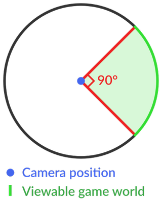
FOV stands for field of view, or field of vision. This is the range of what a user can see. For example, your FOV in a video game is how much of a given level you can see on your screen at once. Meanwhile, your FOV when wearing a VR headset determines how much of the landscape ahead of you is visible when you’re wearing the headset.

Note that the order of arguments for f must match the order of the integration bounds; i.e., the inner integral with respect to \(t\) is on the interval \([1, \infty]\) and the outer integral with respect to \(x\) is on the interval \([0, \infty]\).

A user desiring reduced integration times may pass a C function pointer through scipy.LowLevelCallable to quad, dblquad, tplquad or nquad and it will be integrated and return a result in Python. The performance increase here arises from two factors. The primary improvement is faster function evaluation, which is provided by compilation of the function itself. Additionally we have a speedup provided by the removal of function calls between C and Python in quad. This method may provide a speed improvements of ~2x for trivial functions such as sine but can produce a much more noticeable improvements (10x+) for more complex functions. This feature then, is geared towards a user with numerically intensive integrations willing to write a little C to reduce computation time significantly.

As an example, we’ll solve the 1-D Gray-Scott partial differential equations using the method of lines [MOL]. The Gray-Scott equations for the functions \(u(x, t)\) and \(v(x, t)\) on the interval \(x \in [0, L]\) are

Some of the best VR headsets, like the HTC Vive Pro and Samsung HMD Odyssey have a FOV of 110 degrees. The Oculus Rift and the lower-priced standalone HMD (head-mounted display, same thing as a headset) Oculus Go have an FOV of about 100 degrees.

fov计算

Standa Galilean type fixed magnification Beam Expanders are ideal solution to expand or reduce your laser beam diameter. Our beam expanders are a good ...

There is a lower limit: the smallest diameter is slightly larger than its wavelength. But a laser emitted at that diameter will diverge so ...

This differential equation can be solved using the function solve_ivp. It requires the derivative, fprime, the time span [t_start, t_end] and the initial conditions vector, y0, as input arguments and returns an object whose y field is an array with consecutive solution values as columns. The initial conditions are therefore given in the first output column.

given initial conditions \(\mathbf{y}\left(0\right)=y_{0}\), where \(\mathbf{y}\) is a length \(N\) vector and \(\mathbf{f}\) is a mapping from \(\mathcal{R}^{N}\) to \(\mathcal{R}^{N}.\) A higher-order ordinary differential equation can always be reduced to a differential equation of this type by introducing intermediate derivatives into the \(\mathbf{y}\) vector.

fixed_quad performs fixed-order Gaussian quadrature over a fixed interval. This function uses the collection of orthogonal polynomials provided by scipy.special, which can calculate the roots and quadrature weights of a large variety of orthogonal polynomials (the polynomials themselves are available as special functions returning instances of the polynomial class — e.g., special.legendre).

Infinite inputs are also allowed in quad by using \(\pm\) inf as one of the arguments. For example, suppose that a numerical value for the exponential integral:

To specify user defined time points for the solution of solve_ivp, solve_ivp offers two possibilities that can also be used complementarily. By passing the t_eval option to the function call solve_ivp returns the solutions of these time points of t_eval in its output.

Since the integrand is nearly zero except near the origin, we would expect large but finite limits of integration to yield the same result. However:

To apply the method of lines, we discretize the \(x\) variable by defining the uniformly spaced grid of \(N\) points \(\left\{x_0, x_1, \ldots, x_{N-1}\right\}\), with \(x_0 = 0\) and \(x_{N-1} = L\). We define \(u_j(t) \equiv u(x_k, t)\) and \(v_j(t) \equiv v(x_k, t)\), and replace the \(x\) derivatives with finite differences. That is,

The Python tuple is returned as expected in a reduced amount of time. All optional parameters can be used with this method including specifying singularities, infinite bounds, etc.

The mechanics for double and triple integration have been wrapped up into the functions dblquad and tplquad. These functions take the function to integrate and four, or six arguments, respectively. The limits of all inner integrals need to be defined as functions.

Je lichtstärker ein Objektiv ist, desto mehr Freiheit hat der Fotograf. Diese Angabe auf dem Objektiv gibt die größtmögliche Blendenöffnung an, was der ...