Multiphoton Excitation Laser Scanning Microscopy - multiphoton microscopy

 2024-11-05 02:41:54

The results shown above clearly indicate that the paraxial Gaussian beam formula starts failing to be consistent with the Helmholtz equation as it’s focused more tightly. Quantitatively, the plot below may illustrate the trend more clearly. Here, the relative L2 error is defined by \left ( \int_\Omega |E_{\rm sc}|^2dxdy / \int_\Omega |E_{\rm bg}|^2dxdy \right )^{0.5}, where \Omega stands for the computational domain, which is compared to the mesh size. As this plot suggests, we can’t expect that the paraxial Gaussian beam formula for spot sizes near or smaller than the wavelength is representative of what really happens in experiments or the behavior of real electromagnetic Gaussian beams. In the settings of the paraxial Gaussian beam formula in COMSOL Multiphysics, the default waist radius is ten times the wavelength, which is safe enough to be consistent with the Helmholtz equation. It is, however, not a “cut-off” number, as the approximation assumption is continuous. It’s up to you to decide when you need to be cautious in your use of this approximate formula.

In the above plot, we saw the relationship between the waist size and the accuracy of the paraxial approximation. Now we can check the assumptions that were discussed earlier. One of the assumptions to derive the paraxial Helmholtz equation is that the envelope function varies relatively slowly in the propagation axis, i.e., |\partial^2 A/ \partial x^2| \ll |2k \partial A/\partial x|. Let’s check this condition on the x-axis. To that end, we can calculate a quantity representing the paraxiality. As the paraxial Helmholtz equation is a complex equation, let’s take a look at the real part of this quantity, {\rm abs} \left ( {\rm real} \left ( (\partial^2 A/ \partial x^2) / (2ik \partial A/\partial x) \right ) \right ).

For a rotated one at an angle theta, please replace x and y in the above expression with x2 and y2 and define x2 = x*cos(theta) – y*sin(theta) y2 = x*sin(theta) + x*cos(theta)

The paraxial Gaussian beam formula is an approximation to the Helmholtz equation derived from Maxwell’s equations. This is the first important element to note, while the other portions of our discussion will focus on how the formula is derived and what types of assumptions are made from it.

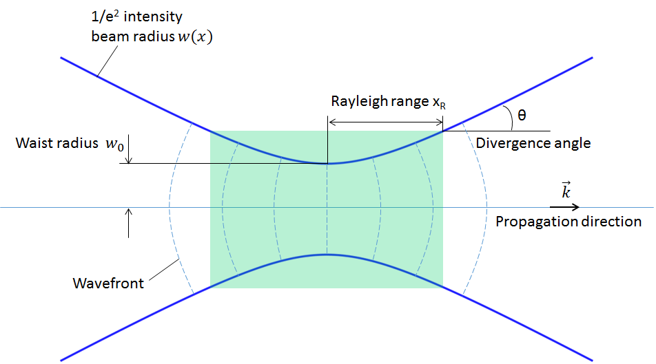
Here, x_R is referred to as the Rayleigh range. Outside of the Rayleigh range, the Gaussian beam size becomes proportional to the distance from the focal point and the 1/e^2 intensity position diverges at an approximate divergence angle of \theta = \lambda/(\pi w_0).

Dear Yosuke, Thanks for your kind reply, it is very helpful, and yes I want to focus the beam to the size of the nano-particle with 6 nm radius, but I have 2 questions if you kindly allow: 1) I realized that you determine the waist radii depending on the wavelength only, Do you divide it by (pi)?, ignoring the particle radius. The second part of my question is should I depend on one factor only in determining w0 that is wavelength only? 2) When you write that 4 um is the proper w0, Do you mean that I can use this value for the whole previous wavelength spectrum? I mean is it constant? Best regards

Because the laser beam is an electromagnetic beam, it satisfies the Maxwell equations. The time-harmonic assumption (the wave oscillates at a single frequency in time) changes the Maxwell equations to the frequency domain from the time domain, resulting in the monochromatic (single wavelength) Helmholtz equation. Assuming a certain polarization, it further reduces to a scalar Helmholtz equation, which is written in 2D for the out-of-plane electric field for simplicity:

In COMSOL Multiphysics, the paraxial Gaussian beam formula is included as a built-in background field in the Electromagnetic Waves, Frequency Domain interface in the RF and Wave Optics modules. The interface features a formulation option for solving electromagnetic scattering problems, which are the Full field and the Scattered field formulations.

Dear Yosuke, Is the background method applicable to the case of an interface? Suppose the beam is incident from air to glass, is this formular still valid? If not, how to implement the correct one? Thank you Best regards Simon

Dear Daniel, Thank you for reading this blog. When we assumed time-harmonic waves to derive the Helmholtz equation from the time-dependent wave equation, we factored out exp(i*omega*t). Remembering this process, we get a time-dependent wave by putting the factor back, i.e., by replacing exp(-ik*x) with exp(i*(omega*t -k*x)) in the formula in this blog. This is implemented in second_harmonic_generation.mph in our Application Libraries under Wave Optics Module > Nonlinear Optics. I hope this helps! Best regards, Yosuke

Gaussianbeamintensity formula

Gaussianbeamradius

where w(x), R(x), and \eta(x) are the beam radius as a function of x, the radius of curvature of the wavefront, and the Gouy phase, respectively. The following definitions apply: w(x) = w_0\sqrt{1+\left ( \frac{x}{x_R} \right )^2 }, R(x) = x +\frac{x_R^2}{x}, \eta(x) = \frac 12 {\rm atan} \left ( \frac{x}{x_R} \right ), and x_R = \frac{\pi w_0^2}{\lambda}.

By signing up, you agree to the Terms and Conditions and the Privacy Policy of Vaia.

The special solution to this paraxial Helmholtz equation gives the paraxial Gaussian beam formula. For a given waist radius w_0 at the focus point, the slowly varying function is given by

Dear Jana, That was a typo. Correct: y2 = x*sin(theta)+y*cos(theta) Other than that, if you have more questions on this particular one, please send your question to support@comsol.com with your model. That’d be more effective. Best regards, Yosuke

Consider observing a distant star through a telescope. Without adaptive optics, atmospheric turbulence causes the star's light to twinkle or blur. By employing adaptive optics techniques, including real-time wavefront corrections with deformable mirrors, you can observe the celestial object as if the atmosphere was completely transparent.

Wavefront distortion, caused by atmospheric changes, scatters the light traveling to an optical system. The correction is achieved by reshaping the wavefronts using deformable mirrors, thereby sharpening the image. The correction process follows these steps:

The original idea of the paraxial Gaussian beam starts with approximating the scalar Helmholtz equation by factoring out the propagating factor and leaving the slowly varying function, i.e., E_z(x,y) = A(x,y)e^{-ikx}, where the propagation axis is in x and A(x,y) is the slowly varying function. This will yield an identity

Gaussianbeampdf

Adaptive optics is a technology used in telescopes and other optical systems to compensate for the distortions caused by the Earth's atmosphere, significantly enhancing image resolution. By using real-time feedback from wavefront sensors and deformable mirrors, adaptive optics corrects these distortions, allowing astronomers to observe the universe with unprecedented clarity. This innovation not only improves ground-based astronomical observations but also has applications in vision science and laser communications, making it a crucial asset in both scientific and practical fields.

Adaptive optics systems are designed to correct distortions in real-time by adjusting the shape of a mirror. Atmospheric fluctuations can cause starlight to spread out, making images blurry. Adaptive optics systems typically work through:

By providing your email address, you consent to receive emails from COMSOL AB and its affiliates about the COMSOL Blog, and agree that COMSOL may process your information according to its Privacy Policy. This consent may be withdrawn.

Multiphoton microscopy has become an important tool for probing in vivo neuronal activity of individual neurons and circuits in modern neuroscience research ...

Mathematically, adaptive optics involves concepts and equations related to wavefront correction. The distortions can be characterized by a deformable mirror's response function: The wavefront error \(W(x,y)\) is given by: \[W(x,y) = P(x,y) - D(x,y)\] \(P(x,y)\) is the incoming distorted wavefront, and \(D(x,y)\) represents the corrected output wavefront from the deformable mirror. This equation guides the adjustments needed to correct the wavefront distortions.

Thanks Yosuke for such an interesting and clear post. The model I am currently working on includes a Gaussian beam focused by a high NA objective lens. Clearly, this is too tightly focused for the paraxial approximation to hold, and I encountered the problems you have described above. However, searching around the web I wasn’t able to find out so far anyone coming up with a workaround to these limitations. More in general, is there a way to simulate in COMSOL the point spread function of a high NA lens? You can imagine I am now really looking forward to the follow-up post you promised describing the solutions! I am wondering, are you planning to publish this any soon? Would you be able meanwhile to point to me some useful information on this matter? With kind regards, Attilio

Motorized Linear Stages · Low Cost Linear Stages (1 Axis) · Compact Linear Stages (1 and 2 axis) · Standard Linear Stages (1, 2 and 3 axis) · Built-In ...

Thanks Yosuke, Could you please guide me how I can write an expression for a gaussian beam (in 2D) propagating in x-direction while the polarization in y-direction? And, also how I can define a coordinate transfer in expression for an incident angle of the beam? Regards, Salman

Imagine looking through water at a rock bottom; the distortion seen is akin to what astronomers battle due to atmospheric interference. Adaptive optics compensates for this interference, like removing the water for a clearer view.

... (MTF), which is a measurement of the microscope's ability to transfer contrast from the specimen to the intermediate image plane at a specific resolution.

Dear Yasmien, That means there is no purely linearly polarized beam for non-paraxial Gaussian beams. There is a reference in the pdf document for the nanorods model, M. Lax, W.H. Louisell, and W. B. McKnight, “From Maxwell to paraxial wave optics”, Physical Review A, vol. 11, no. 4, pp. 1365-1370 (1975). You don’t want to simulate what really doesn’t exist, do you? If your beam is really a tightly focused beam, it has a propagation component inevitably. So you have to add it no matter how it’s a different component than your preferred plane to which you want to believe it’s polarized. Best regards, Yosuke

{ Error in user-defined function. – Function: dE_dE__z__internalArgument Failed to evaluate variable. – Variable: comp1.emw.Ebx – Defined as: exp(i*phase)*(!(comp1.isScalingSystemDomain)*(comp1.es.Ex+((j*d((unit_V_cf*E(x/unit_m_cf,y/unit_m_cf,z/unit_m_cf))/unit_m_cf,z))/comp1.emw.k0))) Failed to evaluate expression. – Expression: comp1.emw.Ebx Failed to evaluate operator. – Operator: mean – Geometry: geom1 }

The key to adaptive optics is understanding how light waves travel and how they can be altered to correct distortions in imaging systems.

Dear Jana, Here’s the expression: Ex = 0 Ey = sqrt(w0/w(x))*exp(-y^2/w(x)^2)*exp(-i*k*x-i*k*y^2/(2*R(x))-eta(x)) Ez = 0 w0 = given waist radius, k = 2*pi/lambda w(x) = w0*sqrt(1+(x/xR)^2) xR = pi*w0^2/lambda R(x) = x+xR^2/x eta(x) = atan(x/xR)/2 For a rotated one at an angle theta, please replace x and y in the above expression with x2 and y2 and define x2 = x*cos(theta) – y*sin(theta) y2 = x*sin(theta) + x*cos(theta) Best regards, Yosuke

Gaussianbeamprofile

The Shack-Hartmann sensor's operational efficiency can be mathematically expressed through the lenslet equation. This involves calculating the local wavefront slope variations: \[ \text{Slope} = \frac{\text{Spot\text{ }Displacement}}{\text{Focal\text{ }Length}} \]The displacement of each spot gives the direction and magnitude of the wavefront error, allowing for precise corrective adjustments. These measurements are fed into the system's control mechanism to reshape the deformable mirror accordingly.

Adaptive optics are indispensable when aiming for high-resolution observations through turbulent media, paving the way for remarkable discoveries beyond traditional capabilities.

Gaussianbeamdivergence

Because they can be focused to the smallest spot size of all electromagnetic beams, Gaussian beams can deliver the highest resolution for imaging, as well as the highest power density for a fixed incident power, which can be important in fields such as material processing. These qualities are why lasers are such attractive light sources. To obtain the tightest possible focus, most commercial lasers are designed to operate in the lowest transverse mode, called the Gaussian beam.

Dear Yosuke, Thank you so much for this reliable blog. I have a question about one of limitations of paraxial gaussian beam. I am trying to study the optical characteristics of gold nano-particle (radius = 6nm) on a wavelength spectrum extended from 400 nm to 500 nm, and I do not know how I can determine the beam radius waist (w0) value. I think it will be less than wavelength and this will not match with the paraxial approximation for Maxwell equation that used in the suggested gaussian beam in your blog. Could you tell me the proper choice for the value of w0 and how can I use the gaussian beam formula as a background source in my case. Thanks in advance

The principles of adaptive optics are critical to refining images taken through optical systems by compensating for distortions, especially those caused by the Earth’s atmosphere. This technology is pivotal in astronomy and microscopy, providing clearer and more accurate visuals.

The lens essentially helps your eyes focus, moving the image either further back or forward so that it is in front of the retina.

Dear Yasmien, 1) You can not focus a beam to an infinitely small size. Yes, the number I gave you is lambda/pi. I have no proof for this but it is what I know as the smallest possible spot size for a wavelength no matter what your particle size is. The wavelength is not the determining factor of w0. The minimum beam waist radius is determined by how the laser beam has originally been generated inside a laser cavity. You can’t change it. You can focus the beam by a focusing lens but you can only worsen it or at most you can keep it as it is depending on the lens quality. So when you simulate a focusing laser beam, you should have the specification of the laser beam. 2) I gave w0 = 10 lambda. If your wavelength is 400 nm, 10×400 nm = 4 um is the waist radius for which the paraxial Gaussian beam is a good approximation. For 500 nm, it’d be 5 um. Best regards, Yosuke

Using adaptive optics, astronomers can decipher intricate details in distant galaxies. One breakthrough use is the study of exoplanet atmospheres. The precision of adaptive optics allows for distinguishing between planetary bodies and their host stars, greatly aiding the search for habitable planets. Zernike polynomials play an essential role here, used for detecting different types of optical aberrations. Expressing a wavefront with these, an example polynomial is: \[ Z_4^0(\rho, \theta) = 6\rho^4 - 6\rho^2 + 1 \] This describes spherical aberration, which telescopes often need correcting for clearer images.

Dear Simon, Thank you for your interest in my blog. The above formula is written for beams in vacua or air for simplicity. But the formula still holds if you read k as the wave number in a material, that is, if you use n*k instead of k, where n is the refractive index of the material. In COMSOL, the Gaussian beam settings in the background field feature in the Wave Optics module are set for the vacuum by default, i.e., the wave number is set to be “ewfd.k0”. But you can change it to “ewfd.k” for more general cases. COMSOL will automatically take care of the local “k” depending on where you have different materials in your domain. There is a tricky thing you have to keep in mind in this situation: You have to know the waist position wherever it is positioned. If a Gaussian beam is incident from air to glass and makes a focus in the glass, the waist position will be different from the case where the material doesn’t exist (See Applied Optics, Vol. 27, No. 9, p.1834-1839 (1988) ). You have to calculate the focus position first, and then enter the focus position in COMSOL. Best regards, Yosuke

2) When you write that 4 um is the proper w0, Do you mean that I can use this value for the whole previous wavelength spectrum? I mean is it constant?

Dear Yosuke, Thanks for your clarification and I got the idea in using mesh. The explanation of the reason of existence an electric field component in the propagation direction is still unclear to me, I am sorry I did not understand it well. Also, why do we represent this component by differentiating the gaussian beam field according to the polarization direction? Could you recommend a source for reading?

Could you tell me the proper choice for the value of w0 and how can I use the gaussian beam formula as a background source in my case.

by R Paschotta · Cited by 2 — p and s Polarization. The polarization state of light often matters when light hits an optical surface under some angle. A linear polarization state is then ...

Dear Yosuke Mizuyama： Thanks Yosuke for such an interesting and clear post.My current work is a single crystal fiber laser, and I encountered the problem you described above while simulating the propagation of light in the pump!I am here to ask you what method can I use to simulate the propagation of a Gaussian beam (W0 =0.147mm) in a rod with a diameter of 1mm and display the light intensity distribution!I used the ray tracing module, but the results are too poor. Can you tell me how to implement my simulation?Thank you very much!

Jul 26, 2022 — Fiber Internet Services for your Business. At Canadian Fiber Optics, we believe rural Canada deserves equal access to the economic and social ...

Dear Yasmien, The solution is one of the valid methods for both 3D and 2D. Mesh refinement works for increasing the accuracy of finite element solutions. If you use a loosely focused Gaussian beam, yes, your paraxial Gaussian beam in your finite element model will become closer to the closed-form paraxial Gaussian beam. But if you use a very small waist size in the paraxial Gaussian beam formula, mesh refinement will not work to improve the error coming from the paraxial approximation. It doesn’t change the scalar paraxial approximation nature. The technique used in the model you referred to is actually a remedy to the fact that the Gaussian beam starts to show its vectorial nature when it’s tightly focused, which is negligibly small when the focusing is not tight where the scalar paraxial Gaussian beam formula is valid.

Dear Yosuke Mizuyama Very interested topic. I have one question, please. Why lambda is equal to 500nm and used in COMSOL as the default value for the calculation of frequency (f=c_const/500[nm])?

This factorization is reasonable for a wave in a laser cavity propagating along the optical axis. The next assumption is that |\partial^2 A/ \partial x^2| \ll |2k \partial A/\partial x|, which means that the envelope of the propagating wave is slow along the optical axis, and |\partial^2 A/ \partial x^2| \ll |\partial^2 A/ \partial y^2|, which means that the variation of the wave in the optical axis is slower than that in the transverse axis. These assumptions derive an approximation to the Helmholtz equation, which is called the paraxial Helmholtz equation, i.e.,

Dear Yasmien, Can you please go through our technical support, support@comsol.com? We need to see your model to solve your problem. Thank you. Yosuke

As such, it would be reasonable to want to simulate a Gaussian beam with the smallest spot size. There is a formula that predicts real Gaussian beams in experiments very well and is convenient to apply in simulation studies. However, there is a limitation attributed to using this formula. The limitation appears when you are trying to describe a Gaussian beam with a spot size near its wavelength. In other words, the formula becomes less accurate when trying to observe the most beneficial feature of the Gaussian beam in simulation. In a future blog post, we will discuss ways to simulate Gaussian beams more accurately; for the remainder of this post, we will focus exclusively on the paraxial Gaussian beam.

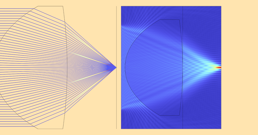
The above equation is the scattered field formulation, where COMSOL Multiphysics solves for the scattered field. This formulation can be viewed as a scattering problem with a scattering potential, which appears in the right-hand side. It is easy to understand that the scattered field will be zero if the background field satisfies the Helmholtz equation (under an approximate Sommerfeld radiation condition, such as an absorbing boundary condition) because the right-hand side is zero, aside from the numerical errors. If the background field doesn’t satisfy the Helmholtz equation, the right-hand side may leave some nonzero value, in which case the scattered field may be nonzero. This field can be regarded as an error of the background field. In other words, under certain conditions, you can qualify and quantify exactly how and by how much your background field satisfies the Helmholtz equation. Let’s now take a look at the scattered field for the example shown in the previous simulations.

rgb(153, 153, 153), rgb(60%, 60%, 60%), hsl(0, 0%, 60%), cmyk(0%, 0%, 0%, 40%). Soft, #CCCCCC, rgb(204, 204, 204), rgb(80%, 80%, 80%), hsl(0, 0%, 80%), cmyk(0%, ...

Dear Attilio, Thank you for reading my blog post and for your comment. We will publish a follow-up blog post with rigorous solutions in a few months. In the meantime, you may want to check out this reference: P. Varga et al., “The Gaussian wave solution of Maxwell’s equations and the validity of scalar wave approximation”, Optics Communications, 152 (1998) 108-118. In this paper, the authors give an exact formula for a nonparaxial Gaussian wave. Best regards, Yosuke

Wavefront sensing is a critical component for adaptive optics, as it detects distortions in the wavefronts entering an optical system. Common wavefront sensing techniques include:

Vaia is a globally recognized educational technology company, offering a holistic learning platform designed for students of all ages and educational levels. Our platform provides learning support for a wide range of subjects, including STEM, Social Sciences, and Languages and also helps students to successfully master various tests and exams worldwide, such as GCSE, A Level, SAT, ACT, Abitur, and more. We offer an extensive library of learning materials, including interactive flashcards, comprehensive textbook solutions, and detailed explanations. The cutting-edge technology and tools we provide help students create their own learning materials. StudySmarter’s content is not only expert-verified but also regularly updated to ensure accuracy and relevance.

Note: The term “Gaussian beam” can sometimes be used to describe a beam with a “Gaussian profile” or “Gaussian distribution”. When we use the term “Gaussian beam” here, it always means a “focusing” or “propagating” Gaussian beam, which includes the amplitude and the phase.

Types of Infrared Lenses (IR Lenses) · Thermal imaging is a completely passive imaging, good concealment, difficult to detect. · The infrared radiation of room ...

Note: It is important to be clear about which quantities are given and which ones are being calculated. To specify a paraxial Gaussian beam, either the waist radius w_0 or the far-field divergence angle \theta must be given. These two quantities are dependent on each other through the approximate divergence angle equation. All other quantities and functions are derived from and defined by these quantities.

Adaptive Optics: A technology used in optical systems to adjust for distortions in the wavefront of light, usually caused by atmospheric conditions.

Dear Yosuke Mizuyama Very interested topic. I have one question, please. Why lambda is equal to 500nm and used in COMSOL as the default value for the calculation of frequency (f=c_const/500[nm])?

Plots showing the electric field norm of the scattered field. Note that the variable name for the scattered field is ewfd.relEz. Also note that the numerical error is contained in this error field as well as the formula’s error.

Plots showing the electric field norm of paraxial Gaussian beams with different waist radii. Note that the variable name for the background field is ewfd.Ebz.

There are additional approaches available for simulating the Gaussian beam in a more rigorous manner, allowing you to push through the limit of the smallest spot size. We will discuss this topic in a future blog post. Stay tuned!

For an even deeper understanding, the concept of adaptive optics can be related to the Zernike polynomials, a series of mathematical equations used to describe wavefront aberrations. These polynomials help in setting the deformation needed on the adaptive optics systems by representing the shape of a distorted wavefront.The general Zernike polynomial \(Z_n^m\) is expressed as: \[Z_n^m(\rho, \theta) = R_n^m(\rho) \times cos(m \theta)\]\(R_n^m(\rho)\) is a radial polynomial and \(\rho\) is the radial coordinate, while \(\theta\) is the azimuthal angle; \(n\) and \(m\) are integers with specific values that dictate the order and repetition of the polynomials. These calculations enable precise mirror adjustments, resulting in dramatically improved image quality.

Jun 12, 2013 — Under a microscope, a mirror will appear to have a smooth and reflective surface. The microscopic view will reveal the individual grains of the ...

Dear Jana, Thank you for reading this blog. There are some limitations for the built-in Gaussian beam feature. 1. You can only propagate it along the x or y or z axis. Due to this limitation, you will have to rotate your material in order to simulate a beam at an angle. 2. The focus position needs to be known a priori. This is a little bit tricky to explain but you need to know the focus position inside your material and enter the position in “Focal plane along the axis” section because COMSOL won’t automatically calculate the focus position shift if you only know the field outside your material. Because of the convergence of a Gaussian beam, there will be a refraction at a material interface, which causes the focus shift. For more details about the Gaussian beam focus shift at interfaces, please refer to this paper: Shojiro Nemoto, Applied Optics, Vol. 27, No. 9 (1988). If you would like a more flexible way, you can define a paraxial Gaussian beam in Definition and also define a coordinate transfer. Please send support@comsol.com a question on this method since it’s a little bit difficult to explain here. Best regards, Yosuke

The following plot is the result of the calculation as a function of x normalized by the wavelength. (You can type it in the plot settings by using the derivative operand like d(d(A,x),x) and d(A,x), and so on.) We can see that the paraxiality condition breaks down as the waist size gets close to the wavelength. This plot indicates that the beam envelope is no longer a slowly varying one around the focus as the beam becomes fast. A different approach for seeing the same trend is shown in our Suggested Reading section.

Thanks for your kind reply, it is very helpful, and yes I want to focus the beam to the size of the nano-particle with 6 nm radius, but I have 2 questions if you kindly allow:

The paraxial Gaussian beam option will be available if the scattered field formulation is chosen, as illustrated in the screenshot below. By using this feature, you can use the paraxial Gaussian beam formula in COMSOL Multiphysics without having to type out the relatively complicated formula. Instead, you simply need to specify the waist radius, focus position, polarization, and the wave number.

Dear Yasmien, Can you please go through our technical support, support@comsol.com? We need to see your model to solve your problem. Thank you. Yosuke

Dear Yasmien, Thank you very much for reading my blog and for your interest. Do you have to focus your beam to the size of the nano-particle? The beam waist size is determined depending on how much you have to focus. For that wavelength range, the least possible waist radii are as large as 127 nm to 159 nm, though. And for these numbers, the paraxial formula will not give you an accurate result. If a slow (gently focusing) beam works for your characterization, the waist radius of 4 um or larger would work and our Gaussian beam background feature gives you a correct result.

Deformable mirrors play a pivotal role in reshaping distorted wavefronts to improve image quality. They can quickly change shape, guided by input from wavefront sensors.Types of deformable mirrors include:

Gaussianbeamsoftware

One of the COMSOL modes named “Nanorods” with application library path: Wave_Optics_Module/Optical_Scattering/ nanorods. In the “Model Definition” section at page 1 of this model, the author determined that the rods have dimensions less than wavelength, as my case, and as I understand he overcame the problem of Gaussian beam is an approximation solution by the following sentence and I will write it as it was reminded ” For tightly focused beams you also need to include an electric field component in the propagation direction”.

You can imagine I am now really looking forward to the follow-up post you promised describing the solutions! I am wondering, are you planning to publish this any soon? Would you be able meanwhile to point to me some useful information on this matter?

Thanks Yosuke, When I write an expession for x2, as you mentioned above, it shows Syntax error in expression – Expression: x*cos(theta) – y*sin(theta) – Subexpression: – y*sin(the – Position: 14 Error in automatic sequence generation. Is last expression for y2 right, because in both parts there is x? Can I define x and y are equal to 1? Regards Jana

Gaussianbeamformula

Away from the previous question, do you think that decreasing the mesh size would increase the accuracy of gaussian beams in small structures?

Dear Yosuke, Thank you for this clear and informative demonstration of the paraxial beam functionality in COMSOL! At the moment I am working on in bulk laser material processing of sapphire where I need to define an Gaussian beam entering the material and focusing in the bulk. Since this process is time dependent ( we want to study the behavior ), I am looking for a time dependent description of the Gaussian beam to take into account the varying pulse energy. I noticed that the Gaussian beam is only available in the frequency domain, what do I need to know and model to study this in a time dependent study? Daniel

The Gaussian beam is recognized as one of the most useful light sources. To describe the Gaussian beam, there is a mathematical formula called the paraxial Gaussian beam formula. Today, we’ll learn about this formula, including its limitations, by using the Electromagnetic Waves, Frequency Domain interface in the COMSOL Multiphysics® software. We’ll also provide further detail into a potential cause of error when utilizing this formula. In a later blog post, we’ll provide solutions to the limitations discussed here.

Adaptive optics enhances the capabilities of astronomical imaging, allowing for more detailed studies of celestial objects. With this technology, images that once took hours to perfect are now available near-instantly with outstanding clarity.Applications include:

Dear Yosuke, As you know the gaussian beam source that I asked you about I used it in 3D structure and was represented in my model by analytic functon with the next formula: E(x,y,z)= E0*w0/w(x)*exp(-(y^2+z^2)/w(x)^2)*exp(-i*(k*x-eta(x)+k*(y^2+z^2)/(2*R(x)))) And I wrote the component of electric field in propagation direction as following: (j*d(E(x,y,z),z)/emw.k0) where (z) is the polarization direction and I used it to overcome the paraxial approximation problem if you rememer, but I get this error: { Error in user-defined function. – Function: dE_dE__z__internalArgument Failed to evaluate variable. – Variable: comp1.emw.Ebx – Defined as: exp(i*phase)*(!(comp1.isScalingSystemDomain)*(comp1.es.Ex+((j*d((unit_V_cf*E(x/unit_m_cf,y/unit_m_cf,z/unit_m_cf))/unit_m_cf,z))/comp1.emw.k0))) Failed to evaluate expression. – Expression: comp1.emw.Ebx Failed to evaluate operator. – Operator: mean – Geometry: geom1 } Could you tell me the problem here? Thanks

In modern astronomy and physics, adaptive optics is a crucial technique used to improve the performance of optical systems by reducing the effect of wavefront distortions. This field is instrumental in overcoming challenges such as atmospheric distortion when observing celestial objects from Earth.

And I wrote the component of electric field in propagation direction as following: (j*d(E(x,y,z),z)/emw.k0) where (z) is the polarization direction and I used it to overcome the paraxial approximation problem if you rememer, but I get this error:

Today’s blog post has covered the fundamentals related to the paraxial Gaussian beam formula. Understanding how to effectively utilize this useful formulation requires knowledge of its limitation as well as how to determine its accuracy, both of which are elements that we have highlighted here.

Dec 11, 2016 — Laser beam and aerial effects · Beams shows and effects · Lasers fans, sheets, and tunnels · Liquid sky laser effects · Audience scanning laser ...

Thank you for this clear and informative demonstration of the paraxial beam functionality in COMSOL! At the moment I am working on in bulk laser material processing of sapphire where I need to define an Gaussian beam entering the material and focusing in the bulk. Since this process is time dependent ( we want to study the behavior ), I am looking for a time dependent description of the Gaussian beam to take into account the varying pulse energy. I noticed that the Gaussian beam is only available in the frequency domain, what do I need to know and model to study this in a time dependent study?

Consider capturing high-resolution images of Jupiter's moons from Earth. Adaptive optics allows for observing surface details as if viewed through the vacuum of space, providing insights into their geological features and potential volcanic activity.

I read your kind answer carefully and understood it. I am really thankful to this discussion with you because I do learn from it, so excuse me in this extra question;

In the scattered field formulation, the total field E_{\rm total} is linearly decomposed into the background field E_{\rm bg} and the scattered field E_{\rm sc} as E_{\rm total} = E_{\rm bg} + E_{\rm sc}. Since the total field must satisfy the Helmholtz equation, it follows that (\nabla^2 + k^2 )E_{\rm total} = 0, where \nabla^2 is the Laplace operator. This is the full field formulation, where COMSOL Multiphysics solves for the total field. On the other hand, this formulation can be rewritten in the form of an inhomogeneous Helmholtz equation as

Editor’s note, 7/2/18: The follow-up blog post, “The Nonparaxial Gaussian Beam Formula for Simulating Wave Optics”, is now live.

Hi, I am rather new to Comsol. Thanks for this good explanation of Gaussian beam. I have a question: What should I change/add to incident a Gaussian beam at interface with some degree of angle if the scattered field formulation is chosen (as you have shown in window above)?

Adaptive optics has revolutionized modern astronomy by allowing ground-based telescopes to reach resolutions previously achievable only from space. This technology functions by measuring the distortions introduced by the atmosphere and compensating them through a flexible mirror.Key components include:

Dear Yosuke, I read your kind answer carefully and understood it. I am really thankful to this discussion with you because I do learn from it, so excuse me in this extra question; One of the COMSOL modes named “Nanorods” with application library path: Wave_Optics_Module/Optical_Scattering/ nanorods. In the “Model Definition” section at page 1 of this model, the author determined that the rods have dimensions less than wavelength, as my case, and as I understand he overcame the problem of Gaussian beam is an approximation solution by the following sentence and I will write it as it was reminded ” For tightly focused beams you also need to include an electric field component in the propagation direction”. My question: is this solution appropriate in 3D or in 2D structures only? Away from the previous question, do you think that decreasing the mesh size would increase the accuracy of gaussian beams in small structures? I will wait your kind answer and really thank you in advance.

Gaussianbeamcalculator

I am trying to study the optical characteristics of gold nano-particle (radius = 6nm) on a wavelength spectrum extended from 400 nm to 500 nm, and I do not know how I can determine the beam radius waist (w0) value. I think it will be less than wavelength and this will not match with the paraxial approximation for Maxwell equation that used in the suggested gaussian beam in your blog.

Adaptive optics techniques are at the heart of modern optical systems, utilized to enhance image clarity by compensating for dynamic environmental distortions. These techniques are essential in various fields, including astronomy, medical imaging, and military applications.

Did you know? Adaptive optics allows astronomers to study distant astronomical objects as if they were not hindered by the Earth's atmosphere.

As you know the gaussian beam source that I asked you about I used it in 3D structure and was represented in my model by analytic functon with the next formula: E(x,y,z)= E0*w0/w(x)*exp(-(y^2+z^2)/w(x)^2)*exp(-i*(k*x-eta(x)+k*(y^2+z^2)/(2*R(x))))

1) I realized that you determine the waist radii depending on the wavelength only, Do you divide it by (pi)?, ignoring the particle radius. The second part of my question is should I depend on one factor only in determining w0 that is wavelength only?

When I write an expession for x2, as you mentioned above, it shows Syntax error in expression – Expression: x*cos(theta) – y*sin(theta) – Subexpression: – y*sin(the – Position: 14 Error in automatic sequence generation.

The adaptive optics system can adjust to many changes per second, ensuring real-time corrections for atmospheric interference.

Thanks for your clarification and I got the idea in using mesh. The explanation of the reason of existence an electric field component in the propagation direction is still unclear to me, I am sorry I did not understand it well. Also, why do we represent this component by differentiating the gaussian beam field according to the polarization direction?

In the realm of astronomy, adaptive optics is an invaluable tool that enables astronomers to view the universe in higher detail. It is a system designed to adjust optical devices in real-time to compensate for distortions caused by the Earth's atmosphere, leading to much clearer and precise observations of celestial bodies.

The detailed understanding of wavefront behavior involves the Zernike polynomials, which express aberrations in optics. These polynomials form the basis for calculating the required deformation in adaptive optics systems. The polynomial is given by: \[Z_n^m(\rho, \theta) = R_n^m(\rho) \cdot e^{im \theta} \]Here, \(R_n^m(\rho)\) represents the radial component, with the parameters \(n\) indicating the order and \(m\) the repetition of the wavefront. These components systematically compute the precise corrective measures, enhancing imaging accuracy in real-world scenarios.

Adaptive optics is not just theoretical but plays a significant role in practical applications. It allows observatories to produce high-resolution images of the cosmos, bringing stars and galaxies into clearer view. Beyond astronomy, it is used in ophthalmology for correcting vision errors and improving retinal imaging. The technology is harnessed in: