Deepdepth of field

Not all products or services are approved or offered in every market, and approved labelling and instructions may vary between countries. Please contact your local representative for further information.

The next level of correction is found in the ‘Plan-Achromatic’ objectives. These are often identified by the abbreviations ‘Plan Achromat’ or ‘Achroplan’ on the barrel of the objective. As well as being corrected for axial chromatic aberration, these objectives are also corrected for an optical phenomenon known as ‘field curvature’. This phenomenon occurs when light passes through a curved lens. The projected image results in curved view of the specimen. If a specimen was viewed using an objective which is not corrected for field curvature, this would result in a non-uniform focus for the whole field of view. Either the edges or the centre of the field of view could be focussed, but not in conjunction.  Although this isn’t generally a problem for routine viewing and checking of specimens, it can be more problematic should you wish to capture images for use in publication for example. In such cases it would be recommended to use plan-achromatic objectives for flat-field correction and uniform focus across the image view.

Depth of field equationexample

At high numerical apertures of the microscope, depth of field is determined primarily by wave optics, while at lower numerical apertures, the geometrical optical circle of confusion dominates the phenomenon. Using a variety of different criteria for determining when the image becomes unacceptably sharp, several authors have proposed different formulas to describe the depth of field in a microscope. The total depth of field is given by the sum of the wave and geometrical optical depths of fields as:

Shallowdepth of field

Microscope objectives are manufactured and corrected to take one or more of these aberrations into consideration within each optical component. Included in the information etched on the barrel of an objective (in addition to magnification, objective type, numerical aperture (NA) and so on) there will be information concerning the optical correction (see Figure 3).

A word on microscope hygiene: if you are using a microscope in a shared laboratory or facility, hygiene and cleanliness are important factors. One important consideration is that of eye infections. If you are unfortunate enough to have an eye infection, you should refrain from using shared microscopes until this has completely cleared up. Eye infections can be highly contagious and are easily spread to other microscope users. Regardless of the health of your eyes, you should always leave the eyepieces and eyecups (and the whole microscope for that matter) in a clean condition ready for the next user.

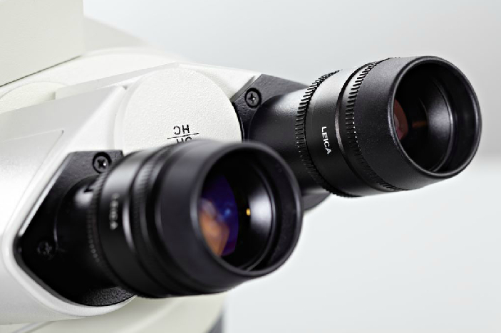
The eyepieces are the optical lenses where we see the final images of specimens (see Figure 1). These optics are sometimes referred to as ‘ocular lenses’ or ‘oculars’. As well as the magnification which is dependent on objective selection, there is an additional magnification factor from the eyepieces to consider which is usually in the order of a 10x magnification. An eyepiece looks like a deceptively simple optical component of the microscope. Whilst it is true that some of the basic eyepieces are comprised of a  a metal tube with lenses top and bottom, many of the research grade eyepieces consist of groups of lenses designed to work in conjunction with each other  to give a corrected view of your specimen as well as complimenting the properties of the objectives.

Depth of field equationcalculator

In addition to the above barrel abbreviations, there are objectives with ‘Plan FL’ or ‘Plan Fluor’ designations. These objectives are corrected not only for spherical and chromatic aberrations but also for field curvature.

Taking into consideration all of the light waves which may pass through a curved lens, the waves which pass through the centre of the lens will be refracted less than the waves which pass through the edges of the curved lens. The light waves which were parallel before passing through the lens do not converge to a single focal point but instead are spread as different points along the optical axis (Figure 3).

Axial resolution, like horizontal resolution, is determined only by the numerical aperture of the objective (Figure 2), with the eyepiece merely magnifying the details resolved and projected into the intermediate image plane. Just as in classical photography, depth of field is determined by the distance from the nearest object plane in focus to that of the farthest plane also simultaneously in focus. In microscopy depth of field is very short and usually measured in units of microns. The term depth of focus, which refers to image space, is often used interchangeably with depth of field, which refers to object space.

Depth of fieldphotography examples

The human eye can normally accommodate from infinity to about 25 centimeters, so that the depth of field can considerably greater than that given by the equation above when one observes the microscope image through the eyepieces. On the other hand, a video sensor or photographic emulsion lies in a thin fixed plane so that the depth of field and axial resolution using those sensors are given by the parameters in the equation. In these cases, the axial resolution is defined by convention as one-quarter of the distance between the first minima, above and below focus, along the axis of the three-dimensional diffraction image produced by the objective.

This interchange of nomenclature can lead to confusion, especially when the terms are both used specifically to denote depth of field in microscope objectives. The geometric image plane might be expected to represent an infinitely thin section of the specimen, but even in the absence of aberrations, each image point is spread into a diffraction figure that extends above and below this plane. The Airy disk, a basic unit of the diffraction pattern produced by the microscope objective, represents a section through the center of the intermediate image plane. This increases the effective in-focus depth of the Z-axis Airy disk intensity profile that passes through slightly different specimen planes.

Depth of fieldphotography

Regardless of the component design of the eyepiece, there are only two lenses at either end of the metal housing which are visible to the user. The lenses through which the final image is viewed (closest to eyes) are referred to as the ‘Eye Lens’, whereas the lens at the opposite end (facing into the microscope body) are referred to as the ‘Field Lens’.

Depth of focus varies with numerical aperture and magnification of the objective, and under some conditions, high numerical aperture systems (usually with higher magnification power) have deeper focus depths than do those systems of low numerical aperture, even though the depth of field is less (see Table 1). This is particularly important in photomicrography because the film emulsion or digital camera sensor must be exposed or illuminated in a plane that falls within the focus region. Small errors made to focus at high magnification are not as critical as those made with very low magnification objectives. Table 1 presents calculated variations in the depth of field and image depth in the intermediate image plane in a series of objectives with increasing numerical aperture and magnification.

Eyepieces need to be adjusted to suit the vision of the user. This is known as ‘diopter adjustment’ and it is used to correct the focal and visual difference between eyes (see Figure 2). Unless you have perfect normal visual acuity (also known as‘20/20 vision’) then making this simple adjustment will allow for sharper and clearer viewing of specimens. Before making the diopter adjustment, a simple physical alteration should be made to the distance between the eyepieces (assuming you are using a binocular microscope) to suit the anatomy of the user. Binocular eyepieces are mounted on a horizontal ‘slider’ and both eyepieces are moved to suit the distance between the eyes. Alternatively, each eyepiece is mounted in separate housing which can be moved in a semi-circular rotation to match the distance between the eyes of the user.

For most microscope applications, there are generally only two sets of optics which are adjusted by the user, namely, the objectives and the eyepieces. Of course, this is assuming that the microscope is already corrected for Koehler Illumination during which the condenser and diaphragms are adjusted.

Once the physical distance is correctly set up, then the dioptre adjustment can be made. If you examine each of the eyepieces, you will note that at least one of them has a knurled ring around the metal body or housing (the other can also be a fixed focus eyepiece). Look down through the fixed eyepiece only and bring your specimen into sharp focus using the main focus wheels of the microscope. Close the eye over the fixed focus eyepiece and look at the specimen using the dioptre adjustable eyepiece only. Whilst keeping the original focus of your specimen, slowly turn the dioptre ring until the specimen comes in sharp focus. When you open both eyes, the specimen should now be in sharp focus. Once the dioptre adjustment has been made, the settings are the same for each objective selected.

Table 1: The International Organization of Standardization (ISO) discriminates three groups of objective classes differing in the quality of chromatic correction: Achromats, Semi-Apochromats and Apochromats. The Leica nomenclature further discriminates these groups according to e.g. their field flatness, transmission etc.

In terms of microscopy (and in the scope of this article), there are two main types of optical aberrations: chromatic aberrations and geometric aberrations. The geometric (also known as ‘monochromatic’ or ‘spherical aberrations’) are also known as ‘Seidel Aberrations’. Philipp Ludwig von Seidel (1821-1896) was a German mathematician, who, in 1857, determined the five constituent geometric aberrations (spherical, coma, astigmatism, distortion and field curvature). In general, the geometric/monochromatic/Seidel aberrations occur due to the structure and geometry to lenses and the way in which light behaves in relation to refraction and reflection when passing through lenses.

In digital and video microscopy, the shallow focal plane in the target of the camera tube or CCD, the high contrast achievable at high objective and condenser numerical apertures, and the high magnification of the image displayed on the monitor all contribute to reducing the depth of field. Thus, with video, we can obtain very sharp and thin optical sections, and can define the focal level of a thin specimen with very high precision.

Depth of field equationpdf

The highest level of corrected objectives (which is reflected in the cost of these optics) are the ‘Apochromatic’ objectives. These are identified by the abbreviations ‘Plan Apochromat’, ‘PL APO’, or ‘Plan Apo’ on the barrel of the objective (see Table 1). These objectives are corrected for field curvature (hence the ‘Plan’ in the abbreviated name) as well as being chromatically corrected for red, green and blue component wavelengths. Furthermore, the apochromatic objectives are also spherically corrected for up to three wavelengths. The high levels of correction found in apochromatic lenses result in higher NA’s compared to equivalent magnifications of objectives with less correction.

Michael W. Davidson - National High Magnetic Field Laboratory, 1800 East Paul Dirac Dr., The Florida State University, Tallahassee, Florida, 32310.

Depth of fieldexamples

An overview of the different classes of Leica corrected objectives can be found by following this link (see Table 1). In addition, Leica can help you to find the exact objective needed for your applications by filling in the on-line form on this page.

Around the eye lens, you will usually find rubber or plastic eyecups (see Figure 2). These serve several functions. They will block out some of the ambient light which gives a clearer view of the specimen of interest. Moreover they constrain users to the optimal distance to the eyepiece. If you wear glasses, they can simply be rolled back over the top of the eyepiece or be removed completely.

Eyepieces and objectives are designed by microscope manufacturers to work in combination and optically complement each other. This is something which should be remembered if, for any reason, you are changing eyepieces or objectives between microscopes. The objectives and eyepieces of a microscope must work harmoniously with each other for optimal specimen imaging. When buying a complete microscope, the optical components will be designed and matched to complement each other to offer optimal viewing conditions for the user. Alternatively, if you are assembling a custom research grade microscope, then the choices of objectives on offer will determine which eyepieces are suitable for the range of objectives and vice versa.

World-class Nikon objectives, including renowned CFI60 infinity optics, deliver brilliant images of breathtaking sharpness and clarity, from ultra-low to the highest magnifications.

These values for the depth of field, and the distribution of intensities in the three-dimensional diffraction pattern, are calculated for incoherently illuminated (or emitting) point sources where the numerical aperture of the condenser is greater than or equal to that of the objective. In general, the depth of field increases, up to a factor of 2, as the coherence of illumination increases (as the condenser numerical aperture approaches zero). However, the three-dimensional point spread function (PSF) with partially coherent illumination can depart in complex ways from that so far discussed when the aperture function is not uniform. In a number of phase-based, contrast-generating modes of microscopy, the depth of field may turn out to be unexpectedly shallower than that predicted from the equation above and may yield extremely thin optical sections.

The next level of corrected objectives are ‘Semi-Apochromatic’ or ‘Fluorite’ objectives. These are identified by the abbreviations ‘Fluar’, ‘Fluor’, ‘Fluo’, or ‘Fl’ on the barrel of the objective. The term ‘Fluorite’ dates back to a time when such lenses were manufactured from fluorite which is a calcium fluoride mineral. Commercially, this mineral is also known as ‘fluorspar’ and is still used in the manufacturing of some of the semi-apochromatic lenses, although most of them are now made from synthetic material. Semi-apochromatic objectives are corrected for one or two component colours and the corrections ensure that the different light waves are focussed together as what is known as the ‘circle of least confusion’ on the optical axis.

When considering resolution in optical microscopy, a majority of the emphasis is placed on point-to-point lateral resolution in the plane perpendicular to the optical axis (Figure 1). Another important aspect to resolution is the axial (or longitudinal) resolving power of an objective, which is measured parallel to the optical axis and is most often referred to as depth of field.

Chromatic aberrations mainly occur due to material of the lens. White light is made up from a number of different wavelengths/colours and when it passes through a convex lens, it is split into its components.  This splitting of wavelengths mean that the component colours do not focus to the same convergence point as each other once the light passes through the lens (Figure 4).

Where d(tot) represents the depth of field, λ is the wavelength of illuminating light, n is the refractive index of the medium (usually air (1.000) or immersion oil (1.515)) between the coverslip and the objective front lens element, and NA equals the objective numerical aperture. The variable e is the smallest distance that can be resolved by a detector that is placed in the image plane of the microscope objective, whose lateral magnification is M. Using this equation, depth of field (d(tot)) and wavelength (λ) must be expressed in similar units. For example, if d(tot) is to be calculated in micrometers, λ must also be formulated in micrometers (700 nanometer red light is entered into the equation as 0.7 micrometers). Notice that the diffraction-limited depth of field (the first term in the equation) shrinks inversely with the square of the numerical aperture, while the lateral limit of resolution is reduced in a manner that is inversely proportional to the first power of the numerical aperture. Thus, the axial resolution and thickness of optical sections that can be attained are affected by the system numerical aperture much more so than is the lateral resolution of the microscope.

Although there are a number of optical corrections available, this article will look at the four most common ones which are likely to be encountered and used. In addition to the eyepieces, objectives can look deceptively simple. The two lenses at either end of the objective are known as the ‘front lens’ which is nearest the specimen and the ‘rear lens’ which is not visible during use as it faces into the body of the microscope. Most objectives comprise of a relatively complex series of lenses each of which complement each other and are designed to correct the otherwise distorting optical aberrations.

This article covers the components of the eyepieces and how to adjust them correctly to suit your eyes. Moving on to the objectives, we will examine optical aberrations and the four most common objectives which are corrected to overcome these anomalies.

The most commonly corrected microscope objectives are the ‘Achromatic’ objectives. These are often identified by the abbreviations ‘Achro’ or ‘Achromat’ on the barrel of the objective. These objectives are corrected for an optical phenomenon which is known as ‘axial chromatic aberration’. This aberration occurs when white light passes through a convex lens. As a result, the white light is split into its’ component wavelengths of red, green and blue. This splitting means that the wavelengths do not converge at the same focal point on the optical axis (see Figure 4).

If a specimen was viewed using an objective which was not corrected for axial chromatic aberration, then coloured fringes would be visible around the specimen as well as a blurring of the image. Achromatic objectives are corrected for two wavelengths (red and blue) which bring these colours to the approximate same focal point as the green wavelength. Furthermore, the spherical aberration of achromatic objectives is corrected for one color.