An Edge ID file with one ROI in each of the center, part-way, and corner zones of the image was used in eSFR ISO so that Batchview, which analyzes the mean of results for each zone, analyzes just one image per zone. (Otherwise you would get the mean of several measurements, which would have a lower variability). The edge ID shown on the right (format: x_y_LRTB) was chosen because the sharpest edge in the manually-focused image was the left edge of the slanted-square two squares to the right of the center. This square (region 3 in the figure below) was used for the analyses on this page.

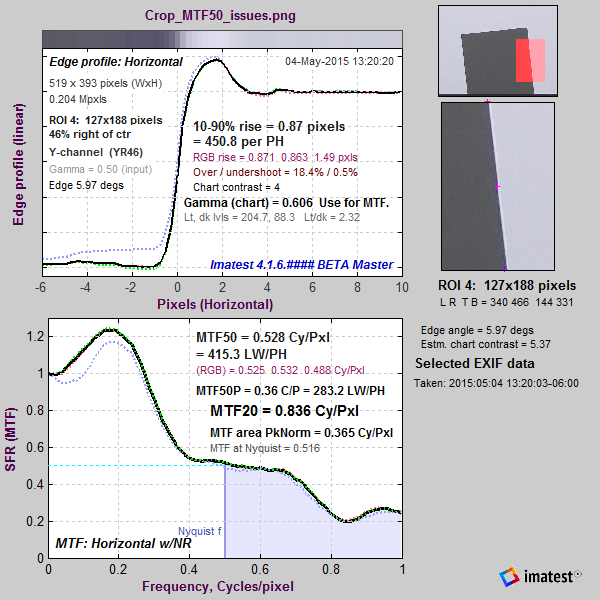
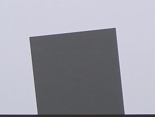
A customer sent us an image whose MTF50 measurements varied unpredictably as ROI size changed. A crop is shown on the right. You can click on it to view a full-sized image that you can download and run.

A key observation (not obvious with normal images, which have much less noise) is that MTF50 is based on the first spatial frequency where MTF drops below 50% of the low frequency level— 997 LW/PH in this plot, where noise causes a sudden and misleading dip just under 1000 LW/PH in the (unsmoothed) MTF curve. Smoothing the MTF plot would improve MTF measurement consistency, but smoothing has never been addressed in the ISO 12233 standard. The optimum amount of smoothing, which depends on the width of the region (i.e., frequency increment or the number of points in the plot) would have to be determined.

The tests were performed on the Panasonic Lumix LX100 camera: a high quality compact camera that has a relatively large sensor, excellent controls, and can produce both JPEG and raw files. We took 10 images of a large eSFR ISO test chart at each of three ISO speeds, saving them in both JPEG and raw formats, for a total of 60 images. (SFRplus could have been used with equally good results.) The lens was set to 50mm-equivalent focal length. Manual focus was used to eliminate variations due to autofocus.  Standard signal processing was selected. A 2-second time delay minimized camera shake.

Proprietary Crosshair Laser Collimator Available With our proprietary laser crosshair, user can zero-in the laser with ease during the final collimation on the secondary and the primary mirror. The crosshair model still exibits a precision laser center dot, but with a touch of four extended laser lines from the center dot. The extension lines (crosshair) of the laser dot is the most intuitive way to guide the laser pointing for an accurate adjustment. During the secondary mirror collimation, a single dot laser projecting on the approximate center of the pre-loaded donut is difficult to identify if the laser dot is exactly on the center.The crosshair laser can easily help user to adjust the secondary mirror to point the laser on the exact center with the help of the crosshair line. During the final primary mirror collimation, the returning laser dot often hides into the laser exiting hole preventing user to identify if the returning laser is at exact center of the hole. Again, the crosshair will visually guide the user to center the laser dot with ease even when the center laser dot disappears into the exiting hole.It is a very effective and essential feature to the SCA Laser Collimator in obtaining at even higher degree of accuracy with ease. Click here for a video tour on YouTube.High Accuracy Laser Alignment

Running the image (using SFRplus with the original uncropped image; SFR with the crop) quickly showed the reason for the problem. A curious combination of excellent lens performance and large sharpening radius (appropriate for a mediocre lens) resulted in a long ramp in the MTF response around the 50% level. Slight changes in response could have major changes in MTF50.

When the system has strong response above the Nyquist frequency, low frequency artifacts such as Moiré fringing or stair-stepping may appear. Stair-stepping is clearly visible when the above image is magnified 5X, as shown on the right. These artifacts have an adverse effect on measurement consistency because an important step in the slanted-edge measurement is the estimate of the edge angle, which is quite consistent for smoothed (anti-aliased) edges, but which depends on the ROI position when there is extreme aliasing. A highly exaggerated example is shown on the far right, where the edge angle estimate derived from the two small red rectangles will be completely different.

In the eSFR ISO Auto mode settings window, all Single-region plots and most Multi-ROI plots were unchecked. (When we needed to examine details we ran eSFR ISO Setup). Close figures after save and Allow CSV file output were checked.

Shipping Policy | Privacy Policy | Return Policy | Imatest Terms and Conditions

This problem will not occur if MTF Area (a relatively unfamiliar summary metric, described below) is used instead of MTF50.

In the eSFR ISO More settings window, MTF plot units were set to LW/PH, Speedup was checked, and MTF noise reduction (mod apod) was checked (except where indicated).

MTF

Keeping the laser dot to the finest point is the key to precision collimation. But when you look closely at the laser dot from brand to brand, most laser dots appear large, not really a fine point as you imagined.This means there is guess work involved when you try to center the dot; not just centering the laser dot to the center of the faceplate, but also centering the center of the dot itself.This does not make any sense when you are trying to take the advantage of the collimated laser beam's characteristic "which has a low beam divergence, so that the beam radius does not undergo significant changes within moderate propagation distances." In other words, the laser beam size within the collimation distance (laser collimator to the primary mirror and back to the faceplate) should remain a constant fine point. As you know, most laser collimator brands are not laser manufacturers.They install an off-the-shelf laser module or pointer and align the laser in a tube without REALLY considering the user’s application, namely the operating distance for a laser beam size.HoTech has been designing and building laser modules and systems for over 20 years for various professional industries.We know exactly how a laser should work.We limit our laser beam to the finest size in the correct operating distance for optimal effect.Our understanding and experiences with the laser design permit you to have an effective and precision collimation.

In summary, our SCA adapter serves three critical functions. First, its expansion rings accommodate almost all focuser's manufacturing tolerances. Second, it automatically centers the adapting laser in the focuser. Third, it provides at least two evenly distributed circular contacts on the focuser's inner tube surface preventing the adapting laser from pivoting and parallel to the focuser.Once the slop factor is taken away, you can quickly collimate your telescope in confidence to achieve perfect collimation every time.Current Collimators' Problems

A second observation is that MTF Area (short for MTF Area Peak-Normalized), which is equal to the integral of the MTF curve from 0 the Nyquist frequency  fNyq, would be closely approximate MTF50 derived from a properly-smoothed monotonically-decreasing MTF curve.

We considered all aspect of parameters in our design.Parameters like the alignment mechanism, mechanical and optical structure of the laser itself, and more are taken as part of our design.For instance, some laser collimators install an off-the-shelf laser pointer in the casing.It is very cost effective (for seller), but it inherits numerous problems.In many cases, the laser pointer might not install perfectly centered in the casing due to pointer size variations and the added alignment mechanism.So the laser itself is not positioned on the true alignment point and optical axis. As the result, the laser can never be center-aligned in the enclosure.It is possible to align the laser beam parallel to the optical path but always with an offset along the optical axis.This means the laser beam is off no matter how you center adapt the laser collimator to the focuser. The result of off-centered laser will introduce astigmatism into your telescope which is similar to figure 1's scenario.

FOV and focal length

As explained in the Sharpening page, the sharpening transfer function is periodic with a period of 1/Radius in Cycles/Pixel. The system MTF (shown on the right for the above image) is the the raw MTF response times the sharpening transfer function.

There may be cases where moderate MTF overshoot (~25-50%) may be desirable. In such cases a modified version of MTF Area may be a better metric. For example (for sharpening between B. and C, above), an image with a spatial domain overshoot of 25% may appear sharper than it would without overshoot— and the halo won’t be very visible. This corresponds to a peak MTF of approximately 1.4.  For a desired peak MTF = MTFpk > 1, we define

The optical axis is shifted when the inserting device is locked in by thumbscrew.In some cases, some poorly made unified compression ring can cause unstable tilt when locking in the drawtube due to loose tolerances between the compression ring, inner groove, and the uneven tip of the locking thumbscrew in a drawtube.The SCA adapts the collimator itself without using the thumbscrew or the unified compression ring.

Another advantage of MTF Area is that it tracks MTF50, i.e., it increases as sharpening increases, up to the point where an overshoot appears in the sharpened MTF curve (peak MTF > 1), then it remains relatively constant. So it does not reward excessive sharpening with better numbers.

LensMTF

The plot below shows the edge and MTF from a raw image captured at ISO 12800. It is extremely noisy because of the very high ISO speed (dim illumination of the sensor, followed by very high gain) and because no noise reduction is applied to raw images.

The pattern of peaks and dips (near 0.42 and 0.84 C/P) suggests a sharpening radius of around 2.4, which would have its first peak around 0.24 C/P. The first system MTF peak is typically lower because of the MTF rolloff of the unsharpened image.

Related page: Correcting Misleading Image Quality Measurements: links to an Electronic Imaging paper that compares MTF summary metrics

In Batchview, enter the […]_sfrbatch.csv output files (from the eSFR ISO batch runs) into boxes A–D at the bottom. Up to four output files can be entered for comparison (though statistical results can only be viewed when a single batch is displayed: Display (lower-right) should be set to A, B, C, or D. The measurement (MTF50, MTF50P, etc.) should be selected from the dropdown menu at the top-left. For this particular analysis, Part way mean was selected in the Region dropdown menu, top-center. (Center mean will be selected in cases where the image is sharpest in the center.) Statistics (mean, sigma) should be selected in the dropdown menu on the top-right (only visible with a single batch is displayed).

Field of view

Many laser collimator manufacturers give users the wrong impression, “big and heavy means rugged and stable.” Instead, HoTech engineers successfully cut the unnecessary weight on the laser collimator because we understand that additional weight on a telescope (especially open structure Newtonians) will create imbalance and structure sagging. The heavier the device is, the more inertia it will have during an impact from an accidental drop.In such an accident, the inertia force can cause more damage to the internal alignment mechanism because there is more energy required to dissipate from the impact.Therefore, the lightweight design on our laser collimator makes you gain reliable precision collimation.And of course our laser collimator uses aero-space grade lightweight aluminum material and CNC machined with the tightest tolerances, then sand blasted and anodized to protect from harsh environment. Nothing has been sacrificed while you get a long lasting state-of-the-art collimation instrument.

This number will be equal to MTF Area for measured MTF peak = 1 (which is the minimum possible value, since MTF is defined as 1 at the lowest spatial frequencies). It will continue to increase up to measured MTF peak = MTFpk, then it will flatten out. For example, for a desired peak MTF = MTFpk = 1.4 (corresponding to spatial overshoot ≅ 25%), MTF Area(1.4) = min(measured MTF peak, 1.4) * MTF Area will reach its maximum when measured MTF peak = 1.4.

Small imperfection inside the drawtube like dents, scratches, and uneven burrs, the rubber rings compensates the errors and faithfully centers the collimator in the tube.In addition, even if the drawtube is slightly deformed in diameter, egg-shaped, the rubber rings in the SCA will compensate the differences and faithfully centers the collimator. A metal collet design will not be able to transform itself to the deformed shape to compensate the imperfection of a drawtube for a sturdy adaption.

Now that these statistical results are available, Imatest will be doing more to promote the use of MTFAPN as a sharpness summary metric.

Our laser collimator is well centered and aligned which are critical factors for an accurate collimation.But you will be surprised that many laser collimators in the market fail in this regard.The reason is in the design and understanding of the product itself.

We propose a new summary metric: the area under the MTF curve (up to the Nyquist frequency), normalized to the peak MTF value. This metric is relatively unfamiliar, but seems to be generally more stable than MTF50 and MTF50P.

Modulation transfer function

This image may look good on the small display of a camera phone, but it is far from optimum when exported and viewed on a large display or printed. When sharpened in this way, image quality won’t approach the potential of the lens and sensor. A better strategy would have been to sharpen with a radius between 1 and 1.5 (perhaps with a moderate oversharpening peak— see sharpening examples, below), then to add additional sharpening for images sent to the display.

The strong response above the Nyquist frequency (0.5 cycles/Pixel)  indicates that the lens is extremely sharp. Images from such lenses tends to look best with sharpening radii well below 2.4, which provides very little response boost in the important 0.35-0.5 C/P range, where the input MTF has sufficient energy to benefit from the boost.

In this page we analyze the consistency of slanted-edge MTF measurements, focusing on the effects of noise and region size on measurement consistency. We describe the test procedure in sufficient detail to enable Imatest users to perform similar studies for themselves.

Note: This page is not quite complete, but we felt that the results are important enough to be presented in its present (nearly complete) state.

ImageJMTF

The targeting faceplate displays the returning laser spot with a clear visual reference during adjustment. That allows you to align your primary mirror from the rear of the telescope and eliminates traveling to the front of your scope repeatedly during collimation.

This is illustrated in the plot on the right, which shows MTF50, MTF50P and MTF Area for an edge (from one of the ISO 200 raw images in the above analysis). The edge was analyzed without sharpening, and with one and two applications of sharpening (Unsharp Mask in Picture Window Pro with Sharpening Radii = 1 and 2). MTF50 continues to increase as sharpening increases, even though the visible effect of sharpening— “halos” near edges— can degrade image appearance. MTF50P increases much more slowly: it’s a generally more reliable metric than MTF50. But it still depends on a single frequency. MTF area does not increase once a sharpening peak > 1 appears.

HoTech understands the importance of this, so the faceplate is a standard feature in our laser collimator.All astronomers deserve to have it without paying any extra!Also, our faceplate viewer’s pattern is laser engraved to ensure a long lasting sharp targeting grid for best visual effects. Unlike other collimators, the target is not a sticker that will peel, or paint that can rub or chip off. We understand that you are paying for a precision instrument that is supposed to be well made.

In running eSFR Auto, select batches of files to be analyzed together, i.e., don’t mix different ISO speeds or JPEG and raw, unless there is a specific need to do so (for example, for directly comparing different ISO speeds). No additional settings need to be entered, since they were saved during eSFR Setup (Rescharts).

MTFtesting Mastercard

All drawtube have manufacturing tolerances.And it requires larger diameter to accept various eyepieces and adapters.When a standard collimator is inserted, the gap between the drawtube and the inserting device became a slop problem.The rubber rings in the SCA expand radially according to users own adjustment to fill the gaps.This makes your collimator seats firmly in your drawtube becoming part of your telescope for a secure and repeatable installation.

A 25×40 pixel region size is sufficient for good results with low noise images. This may be the best that can be done with low resolution cameras, though larger is recommended if the geometry allows or if the image is very noisy.