Understanding camera lenses - understanding camera lenses

 2024-08-22 07:25:02

The spatial profile of the image is called the line spread function (LSF) if the scanning is one-dimensional, or the point spread function (PSF) for two-dimensional scanning. An LSF is commonly produced by edge-scanning an image of a point source with a mechanical obscuration (knife-edge) while monitoring the intensity throughput, and then differentiating the output. It can also be produced by using a slit source and moving a pinhole or slit. The vertical or horizontal orientation of the knife determines whether sagittal or tangential scanning is achieved. If the knife-edge possesses a right angle (often called a “fish-tail”) and is diagonally traversed across the image, it will sequentially scan in the horizontal and vertical directions, yielding both sagittal and tangential edge traces. The Fourier transform of the LSF is the one-dimensional MTF.

Klimasewski, Robert G. A Knife Edge Scanner to Measure The Optical Transfer Function Thesis, University of Rochester, 1967

Lens MTFdatabase

The presence of aberrations reduces the Strehl ratio below its ideal value of 1. For small aberrations the Strehl ratio is given approximately by:

For most optical systems and components measured today, interferometric testing can provide much information about the lens under test, but may not provide full characterization regarding use in the final environment. For this information, Geometric Lens Measurement is required.

As the table shows, the wide variety of optical systems have an equally wide number of required measurements. In recent years, there has been an emphasis placed on wavefront (interferometric) testing for characterization of optics. This is certainly warranted for the highest quality diffraction limited laser systems, but is inappropriate for many optical systems, particularly those requiring polychromatic wide field imaging.

The characterization of the performance of optical systems and components today has become as difficult a task as their actual design and manufacture. The increasing number of optical and mechanical specifications, combined with the more exacting nature of optical design in recent products, are driving the demand for highly detailed measurements.

Over the past 25 years, the concept of the optical transfer function (OTF) has gained popularity. The advent of the computer made both design and testing using OTF and MTF (the magnitude of OTF) a reality: lens design programs can now readily predict polychromatic OTF for a completed optical system and match the results against new measurement equipment.

MTF lenstest

A closed form integration which decomposes spatial energy information into a series of sinusoidal functions which describe frequency content (frequency spectrum). The Fourier transform integral for a complex function g(x, y) is given by:

Second, MTF can be specified either at a single wavelength or over a range of wavelengths, depending upon the application. Interferometric wavefront metrology is limited to certain laser wavelengths. MTF allows full spectrum specification and testing.

This guide is designed to provide insight into the theory and practice of measuring the Modulation Transfer Function and related quantities. While a guide of this size cannot begin to address all the intricacies and subtleties of testing, it is intended to provide a foundation for understanding, and to introduce the reader to the fundamentals of testing. Various tests and test techniques are described in detail and in concept.

This is simply the ratio of the area under the MTF curve to the area under the diffraction limited MTF curve. By Parseval’s theorem this is also the ratio of the irradiance in the center of the diffraction pattern to the center intensity of a diffraction-limited Airy disk.

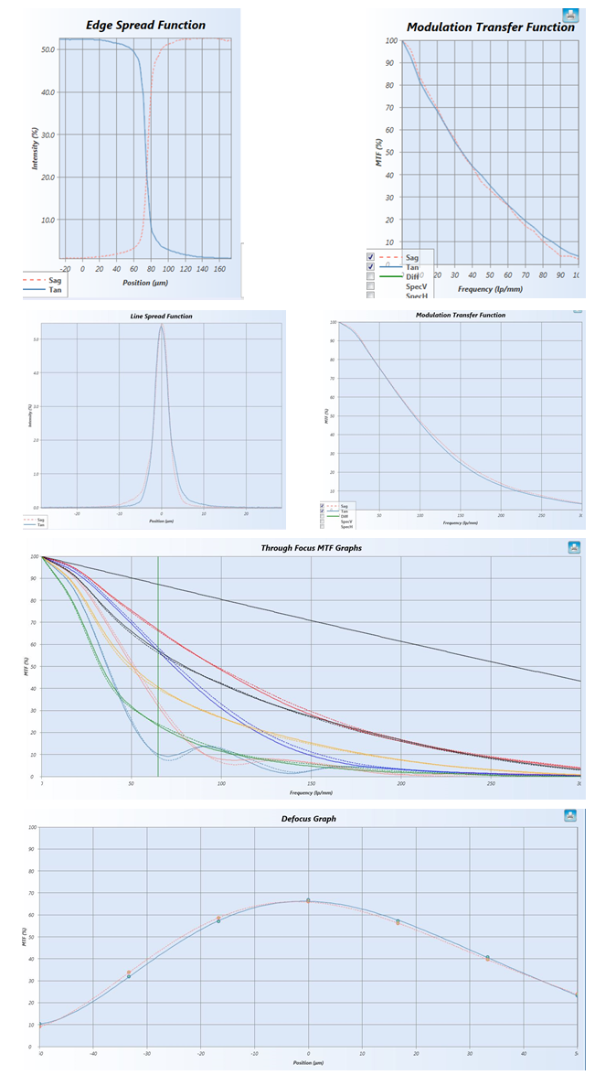
The figure below shows plots of Edge Spread Function (ESF), Line Spread Function (LSF), Modulation Transfer Function (MTF), Through Focus MTF (THF MTF), and defocus MTF (DEF MTF) obtained with scanning and video based metrology systems.

Back or Flange Focal Length - The distances from the rear lens vertex or some mechanical surface to the focal plane are the back and flange focal lengths.

Through-focus MTF mapping can be generated by re-measuring the MTF at different focus planes. The effects of spherical aberration, defocus, astigmatism, field curvature and chromatic aberration can be determined from these curves. By choosing a single spatial frequency and comparing the MTF at these focal planes, the focus for best (or balanced) performance can be determined. The last two frames of Figure 5 show the benefits of through-focus scanning.

Field Curvature - The amount of required refocus of the image as a function of angle is the field curvature. Sagittal and tangential curvatures can be individually monitored by inserting slits in the lens pupil. The lens must be properly Gaussed for field curvature measurement.

Since MTF testing is performed on the image or wavefront produced by an optical system, the parameters which influence lens performance and design can be recreated exactly in the test of the lens. Field angle positions, conjugate ratios, spectral regions, and image plane architecture can all be modeled in the test of an optical system. For example, the characterization of a double Gauss lens at finite conjugates can be easily performed and compared to design expectations or application requirements.

In its simplest form, resolution testing takes the form of an ophthalmic chart — a series of figures, each representing various spatial detail levels, is placed on a page and viewed. In addition to the detail levels, the orientation of the figures (for example, the large letter ‘E’ on the ophthalmic chart) can supply information on the astigmatism of the observer.

The T-Bar maintains flat-plane imaging as the lens is rotated off-axis. The image conjugate (the distance between the rear nodal point and the rear focal point) will lengthen by a distance given by the expression below:

The relatively few drawbacks of video methods are inherent in the design of electronic solid state arrays. Since detector element sizes are finite and on the order of a few microns, the maximum resolvable frequency is approximately –100-200 lp/mm. This problem can be circumvented by adding an optical relay system to magnify the image onto the array. However, the relay optics must be very high quality, must have a very high numerical aperture to capture the entire output of fast lenses or systems working at high off-axis angles, and should be essentially diffraction limited to not impact the measured MTF.

Resolution relates to detectability. The resolution required of a visual optical system is different than for photographic optical systems, for example. Resolution specifications are therefore specified for each application.

Most optical systems are expected to perform to a predetermined level of image integrity. Photographic optics, photolithographic optics, contact lenses, display systems, AR/VR optics, and automototive lenses are just a few examples in the long list of such optical systems. A convenient measure of this quality level is the ability of the optical system to transfer various levels of detail from object to image. Performance is measured in terms of contrast (degrees of gray) or modulation, and is related to the degradation of a perfect point source as it is imaged by a lens.

The third benefit of MTF testing is that it is objective and universal. The test engineer is not required to make judgments of contrast, resolution or image quality. Therefore, under the same conditions the polychromatic MTF of the lens can be directly compared to the polychromatic MTF of a design, or to another measurement instrument.

MTF specifications are frequently used for lens designs that require repeatable test standards. Some examples are reconnaissance lenses, photographic objectives and IR systems. The MTF measurement instrument is also commonly used as a production quality control tool, since operators are not required to have a high level of optical training in order to properly test the optics.

Nelson, C.N., Eisen, F.C., and Higgins, G.C. “Effect of Nonlinearities when Applying Modulation Transfer Techniques to Photographic Systems” Modulation Transfer Function, Proc. S.P.I.E. 13, 127-134, 1968

A drawback to image scanning methods is the duration of scan. Sampling theory and the parameters of the Lens Under Test dictate the number of data points required for a properly sampled image. Insufficient sampling can significantly affect the accuracy of the MTF. Often, a long image scan will require upwards of 30 seconds measurement time.

As an example, consider measurement of a photographic telephoto lens for a 35mm camera. A monochromatic interferometric test of the optical system at the working conjugates will provide information regarding the emerging wavefront characteristics. However, the pertinent information required is the polychromatic performance of the objective over a substantial object field (a 35mm format negative), a good measure of the system’s distortion, the blur quality (size and shape) on-axis and off-axis, an accurate measure of the focal length, and the integrated polychromatic resolution ability of the lens. It is very difficult to configure an interferometer for the wide field geometric measurements desired.

Gerchman, MC. “Testing Generalized Rotationally Symmetric Aspheric Optical Surfaces Using Reflective Null Compensating Components.” Proc. S.P.I.E., 676, 60-65, 1987

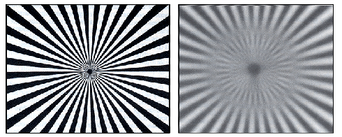
Phase reversals occur when the modulation (and the PTF) changes sign. In this case, whites turn black and blacks turn white. The classic example of Phase Reversal is a radial target with alternating black and white “pie” segments, viewed through a somewhat Defocused (but otherwise perfect) lens. At a certain radial distance from the center the contrast disappears, and the color is a uniform gray. Within that circle the black and white segments are the reverse of what they are outside that circle.

The real portion, or |H(fx,fy)| is called the Modulation Transfer Function, or MTF, and the function Φ(f) is termed the Phase Transfer Function. The MTF is normalized to unity at zero spatial frequency

DeVelis, John B. and Parrent, George B. “Transfer Function for Cascaded Optical Systems” J. Opt. Soc. Am., 57, (12), 1486-1490, 1967

A single number representation for the quality of a lens based on a photographic application. The SQF is derived from the logarithmic integration under the MTF curve in the final image plane. The actual limits of integration are computed by the magnification of the image plane to the final format’s size.

where IMax is the maximum intensity produced by an image (white) and IMin is the minimum intensity (black). MTF is a plot of contrast, measured in percent, against spatial frequency measured in lp/mm. This graph is customarily normalized to a value of 1 at zero spatial frequency (all white or black).

Modulation transfer function

The accuracies required in these two examples illustrate the versatility that is available in Geometric Lens Measurement instrumentation. In the first example, the image is compared to the properties of photographic emulsion or sensor arrays, while a scan lens normally requires high precision for all the measurements. A 5% variation of a singlet focal length (typical catalog specification) compounded five times in a multi-element system can easily cause the magnification to vary 20%. Instrumentation must be able to measure lens parameters with this large variation to the same accuracies (e.g. 1% on efl) of the f-theta lens, which may exhibit a 2% total variation. This describes the inverse relationship between Geometric Lens Measurement and image quality: the poorer quality optics require more from Geometric Lens Measurement instrumentation than higher quality or diffraction-limited optics.

When an optical system produces an image using perfectly incoherent light, then the function which describes the intensity in the image plane produced by a point in the object plane is called the Impulse Response Function. This impulse response usually is written h(x,y; x1,y1). The input object intensity pattern, f(x1, yx1) and output image intensity pattern, g(x, y) are related by the simple convolution equation:

Computer algorithms quickly correct measured MTF data for finite aperture sizes (slits, pinholes, etc.). The fully corrected data can then be compared to the theoretical performance.

One can cascade the MTFs of different system components, provided that all the cascaded systems are linear. In other words, the systems can be cascaded if the response at a particular frequency is linearly proportional to the input signal amplitude. This will be the case with photographic film near the middle of the H-D curve, but not at the ends, or with a CCD at moderate illumination levels, but not near saturation.(Nelson, Eisen, and Higgins 1968)

More details on MTF and the role of MTF measurements on the characterization of optics, including UV and IR optics, appear in the article, “Lens Testing: The Measurement of MTF which follows this article.

Further inquiries regarding test theory, general test techniques and application specifics should be directed to Optikos Corporation. Optikos is the leader in the area of MTF measurement technologies and offers a full product line designed to meet virtually all measurement requirements.

There are two basic categories of commercially available instruments dedicated to measurement of MTF of optical systems using image analysis: physical scanners and video scanners.

Interferometers treat the system in much the same manner. Instead of using the theoretically determined OPD maps as the input, however, phase measurements obtained from an interferometer provides the input. Software algorithms are then used to perform an autocorrelation of this phase map with itself to produce the OTF.

The table below outlines methods for obtaining the Edge Spread Function (ESF), Line Spread Function (LSF), Modulation Transfer Function (MTF), Through Focus MTF (THF MTF), and defocus MTF (DEF MTF) in scanning and video based metrology systems.

Virtually all lens design software today allows graphical depiction and subsequent tolerancing of polychromatic MTF. Lens design software programs calculate the system MTF either through the autocorrelation of the exit pupil wavefront function or by Fourier transforming the point spread function, which is calculated by Fourier transforming the pupil wavefront. Polychromatic MTF is computed by vector addition of the monochromatic MTF and phase function. These methods for calculating MTF are also used with phase measuring interferometers to calculate the MTF of relatively well corrected monochromatic optical systems.

Most commercial instruments dedicated to measuring MTF readily determine polychromatic MTF. The test spectrum can be tuned to the polychromatic design spectrum using photopic filters, infrared bandpass filters, or color filters, for example. Glass substitutions which share the same index of refraction at one wavelength but have different dispersions can severely affect performance of a polychromatic optical system. Monochromatic testing of such a system may not uncover the substitution; polychromatic MTF testing will expose the fabrication error.

Very high resolution (without image magnification) can now be achieved with scanning systems equipped with precision lead screws driven by stepper motors or accurate synchronous motors.

The six “points” of a well-corrected optical system which allow its characterization as a “black box”. The six points are: front and rear focal points, front and rear nodal points, and front and rear principal points. (In most cases of interest, where the medium on either side of the lens is the same, the principal points coincide with the nodal points).

Under appropriate conditions, the MTF of a system can be calculated by “cascading” the MTFs of the component systems. In other words, one can construct the MTF of the composite system at any frequency by multiplying together the MTFs of each of the components at that same frequency:

The discussion above has assumed that the imaging has been performed using an incoherent light source. This is generally the most useful type of measurement, since most imaging applications use incoherent light (natural sunlight, tungsten bulbs, etc.) For the case of incoherent illumination the impulse response function relates the object intensity to the image intensity. The Optical Transfer Function is the Fourier Transform of this impulse response function.

A measure of the irradiance distribution across the image plane produced by a small source object. GSF is typically measured using a bright object in an otherwise dark (black) field, as described in the specification document ISO 9358 and this article.

Modulation Transfer Function (MTF) has been associated with the measurement of the performance of optical systems since the initial introduction of linear system analysis to the field of optics. As the demand for higher quality, higher resolution optical systems became prevalent, both designers and metrology scientists began investigating MTF as a standardized method of optical system characterization. This article serves to identify the reasons for specification and measurement of MTF as a system characterization tool.

The advantage of video MTF measurement lies in the speed with which it can be accomplished. The MTF can be updated as quickly as the solid state array can be electronically sampled and the Fourier transform calculated. This provides a continuously updated spread function and MTF curve.

Function describing the variation of relative phase in the image of an optical system as a function of frequency. It is derived from the imaginary portion of the OTF:

The MTF can be described as a map of modulation versus spatial frequency of a spatially varying source. The spatial frequency is defined as the inverse of the spatial period of the sinosoid.

MTFimage quality

Virtually all nodal testing is accomplished on nodal benches -- instruments designed to locate and position the lens-under-test relative to its cardinal points. All lenses have three pairs of cardinal points: front and rear focal points, front and rear principal planes, and front and rear nodal points. Figure 2 depicts a classic nodal bench.

The figure about shows the additional distance from the lens to the image as a function of field angle. The axial image conjugate, di is defined by the formula below:

Optikos Corporation 107 Audubon Road, Bldg. 3 Wakefield, MA 01880 USA +1 (617) 354-7557 Privacy Policy YouTube LinkedIn X

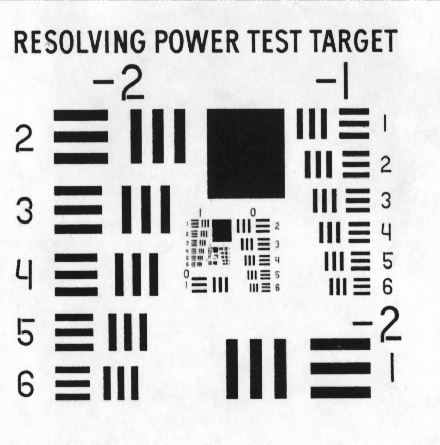
The Aerial Resolution Chart, better known as the 1951 Air Force Chart, is a series of vertical and horizontal bars, spaced with a 50% light-dark duty cycle, wound into clusters of groups and elements. A mask of this chart is used as an object in the nodal bench. The lens under test is positioned to create a real image of the resolution chart, which is examined by the operator under high magnification. The spatial frequency is related to the group number and element number on the chart by the relationship:

The resolution target provides valuable information regarding the resolution characteristics of a lens. Unfortunately, it does not provide discrete methods for discerning relative levels of contrast. High resolution does not always equate to high contrast! Contrast, or ‘modulation’, is the relationship between the maximum intensity and the minimum intensity of the image (dark-light) or the degree of grey.

The primary benefit of Geometric Lens Measurement is that the optical system is tested in the exact same configuration in which it is used. Whether it is an infinite conjugate system or a finite conjugate system (fixed object distance), flat plane or curved, on-axis or vignetted off-axis, wide open or stopped down, the image is produced under exactly the same set of conditions as when it is in use. Polychromatic testing is accomplished with the simple addition of appropriate filters.

Optikos® testing and image quality services are provided through our optical metrology lab and offer the most comprehensive modulation transfer function (MTF) lens testing and imaging sensor testing, as well as non-imaging measurements and optical element information available–all in one location.

There are several methods for measuring MTF -- discrete or continuous frequency generation, image scanning, and wavefront analysis. Recent advancements in precision mechanics and electro-optics technologies have produced many practical variations on these methods that allow efficient measurement of OTF to very high accuracy. Four major categories of instrumentation exist: frequency generation, scanning, video and interferometric methods.

The spatial frequency at which the transferred contrast of a diffraction limited (aberration free) optical system is reduced to zero. For a circularly symmetric diffraction limited system, the cutoff frequency fc is defined as:

The condition of an optical system which describes space invariance. An optical system is said to be space invariant if the image of a point source changes only in location, and not in shape, as the point source is moved in the object plane.

The curvature of the image plane caused by the indices of refraction and curvatures of the optical elements. In the absence of astigmatism only Petzval curvature exists.

An optical instrument which allows determination of the cardinal points of a lens utilizing the principal that a ray which passes through the first nodal point is imaged to the second nodal point at unit magnification and hence exits the lens at the same angle as the entering ray.

Quartz-Silica Wedge Depolarizer Leysop can provide these components in whatever diameter, thickness, number of sections you require (we have manufactured 22 section Lyot depolarizers for one especially critical application) and with or without AR coatings, as you prefer. Components can be provided mounted in protective rings or supplied bare. Please email us for your specific requirements.

The benefits of using MTF as both a design and manufacturing tool lie in its objectivity. Full polychromatic testing of a wide variety of optical systems is possible using MTF testing methods such as edge scanning, video and discrete frequency targets. The MTF can be used to characterize the most demanding and precise optical systems, from photo- lithographic to ophthalmic.

The case of partially coherent light is much more complex. Instead of working with either the complex amplitude of the light or its intensity, we must measure a property called the mutual intensity, and the relevant transfer function describes the propagation of the mutual intensity through the optical system. A discussion of this is beyond the scope of this article. The interested reader is directed to sources such as Born and Wolf’s Principles of Optics, chapter 10.

Also known as Knife Energy Distribution. The map of the intensity of an image as a function of position (frequently normalized) of an obscuring knife blade slid through the image (also known as edge spread function, or ESF).

we can use the last equation above to derive Φ(fx) = -πfxX 0,confirming that a linear shift in position leads to a corresponding linear shift in phase.

A series of MTF measurements made over a range of positions in the vicinity of the focal point. It is used to analyze how the MTF varies with focus position.

Lens MTFcomparison

Cutoff resolution is defined as the frequency at which the contrast of an image is reduced to zero. In other words, it is frequency at which the MTF drops to zero.

The phase transfer function (PTF) describes the relative phases of the sinusoids of different frequency making up the transform. A non-zero phase indicates shift and/or repetition in the image. For example, consider a one-dimensional system in which the response to a delta function object is an image that consists of two spots in the image plane separated by a distance x0. Since the input object is a point or impulse, this image is the impulse response, and the Fourier Transform of it is the Optical Transform Function (OTF).

where G(fx,fy), F(fx,fy), and H(fx,fy) are Fourier Transforms of g(x,y), f(x1,y1), and h(x,y;x1,y1).The function H(fx,fy) is called the Transfer Function, and in the case of optical systems, it is the Optical Transfer Function, or OTF.

Other methods of determining lens quality include star, Ronchi, and knife-edge testing. These established techniques for examining blur patterns reveal many pertinent properties of the lens, such as decentered or tilted internal components, in addition to the types and amounts of aberrations present.

The simplest case is a sine wave. In order to properly sample sine wave of frequency f, we must gather data at a frequency of at least 2f. A common interpretation is that this enables proper sampling of the wave by enabling the measuring device to observe one wave and one trough.

The MTF is a measure of the ability of an optical system to transfer various levels of detail from object to image. Performance is measured in terms of contrast (degrees of gray), or of modulation, produced for a perfect source of that detail level.

Blur Spot Size and Shape - The blur is measured using the reticle cross hairs of the microscope. For example, Airy disk ring diameters and the amount of astigmatism can be directly measured using this technique. The length and separation of the sagittal and tangential lines of an astigmatic image can be found by defocusing the image plane to concentrate upon each individually.

It is sometimes necessary to ensure that a source is completely free of any preferred plane of polarization. An example of this is a sensitive spectrometer where varying degrees of polarization will lead to measurement errors. Of course, in nature almost all sources exhibit some degree of polarization; even thermal sources become polarized after reflection from a dielectric surface. Depolarizers are therefore essential items to have wherever a completely un-polarized source must be used.

The autocorrelation of a wavefront (as given by the pupil function of the optical system) will yield the OTF of a coherent optical system. This technique is commonly used in interferometers and lens design programs. The pupil function is autocorrelated (convolved with itself) to yield the OTF.

Video methods are subject to the same theoretical considerations as the scanning methods. Typically, a solid state array is placed at the focal plane of the lens-under-test (or at the long conjugate of a magnifying relay lens, as described below). If a pinhole source is used, the point spread function can be directly obtained from the digitized video output. The two-dimensional OTF is obtained by directly Fourier transforming this data in two dimensions. Edge traces and line spread functions can be obtained by integrating the point-spread function. If a slit source is used, the line-spread function is obtained directly and the OTF is calculated by performing a one-dimensional Fourier transform of this. In either case, the MTF is given by the modulus of the OTF.

The obvious advantage of frequency generation methods is the fact that the output is directly measured. The major disadvantage is that these methods require the simultaneous manipulation of sources and detectors, which limits instrument flexibility.

Lens MTFchart

Since the object input is a point, a perfect impulse, the transfer function is simply the Fourier Transform of the image function. This is given by:

Depolarization is obtained through the production of varying amounts of circular and elliptical polarization states at different wavelengths. The depolarization effect is poor for monochromatic light as even with a large number of plates in the stack there are only a limited number of polarization states produced. By contrast, a polychromatic source will produce an effectively infinite number of polarization states and thus depolarization is strong, even with just two plates.

The amount of detail in an image is given by the resolution of the optical system, and is customarily specified in line pairs per millimeter (lp/mm). A line pair is one cycle of a light bar and dark bar of equal width and has a contrast of unity. Contrast is defined as:

With the growing role played by optical devices in measurement, communication, and photonics, there is a clear need for characterizing optical components. A basic and useful parameter, especially for imaging systems, is the Modulation Transfer Function, or MTF. Over the past few decades technological advances, including the laser interferometer, high-speed imaging devices (CCD and CMOS Cameras), and advanced computer algorithms have revolutionized the measurement and calculation of MTF. This has made what was once a tedious and involved process into virtually an instantaneous measurement.

Lyot depolarizer, available in Quartz, calcite etc. Lyot depolarizers can be manufactured in just about any birefringent material, but most applications are covered by either quartz or calcite. Quartz is particularly suitable for applications extending into the ultra-violet and we can provide optically contacted components for minimum insertion loss. For applications where calcite is more suitable, we can provide either cemented or even air spaced components (but calcite is not suitable for optical contacting).

There are two principle methods of producing depolarization but they operate in different manners. It is essential that the correct type is chosen based on whether the source is mono- or poly-chromatic.

Non-image-forming light, concentrated or diffuse, that is transmitted through the lens to the image. It is frequently the result of reflections from lens surfaces, a lens barrel, shutter, or lens mount. (See also Veiling Glare and Glare Spread Function.)

Today’s new technologies for designing and producing complex, high quality optical systems require lens measurement equipment that is sophisticated, flexible and accurate

FIGURE 1. Early MTF measurement instruments (circa 1990) allowed full freedom to create a test environment exactly as the design environment, including spectral filtering, off-axis evaluation, conjugate matching, and image plane movement.FIGURE 2. Modern MTF measurement instruments like the Optikos OpTest Bench pictured above maintain the same freedom to create test environments that match the design and application environments, and add the flexibility of automated measurement routines for improved speed, accuracy and repeatability.

Strehl ratio is sometimes improperly used to identify the “percentage of diffraction limited performance” of an optical system, sometimes called XDL, or “Times (“X”) the Diffraction Limit”. The relationship between the Strehl ratio and the “XDL” value relies upon the assumption that aberrations act to broaden the size of the diffraction spot, having no other effect. This is not, in fact, true. It is approximately true if the aberrations are small. In general, however, this term does not compensate for full conditions of the tests and should be context-limited.

Video capture of image data can be used for rapid measurement of the Point Spread Function, from which the MTF can be calculated. In this case there is no knife edge. The relay optic sends a magnified version of the image directly onto the CCD array. This acts like a series of detectors which discretely sample the entire image in one action.

If the functional form of data that we wish to measure has no components beyond a certain frequency, then that function is said to be bandwidth limited. The function can be re-created exactly from a finite series of discrete measurements, provided these measurements meet certain criteria. In order to recreate a function from a series of data points, the measuring system must sample that data at a rate greater than twice its maximum frequency. This frequency (twice the maximum frequency of the sample) is called the Nyquist frequency.

For example, video imaging systems must be designed to consider the image size produced by the lens relative to the array pixel size and location. An array pixel width of 6 microns corresponds to a Nyquist frequency of 83 lp/mm (half the sensor cut-off frequency of 166 lp/mm). In most cases, attempting to resolve beyond this limit is impossible; therefore designing a lens which maintains high MTF out to the Nyquist frequency is appropriate for this application. Specifying performance of a lens beyond this frequency is superfluous.

Here Imax is the maximum intensity in the image and Imin is the minimum intensity. Intensity is measured as W/cm2 (irradiance) by a detector or by video image from a digital camera.

Knife-edge (or Foucalt) and star testing methods have been well established over the past few decades. Star testing is the visual examination of the image produced by the lens of a point source and was the basis for the development of the nodal bench. During the star testing procedure, the departure from a perfect diffraction pattern (Airy disk rings) or coloring of the image indicates to a trained observer the presence of aberrations. The operator can then characterize and quantify the combinations and relative contributions of the aberrations.

The resolution for a real image-forming optical system (a microscope objective or an eyepiece, for example) is again specified by asking an observer to identify the point at which a bar chart becomes unresolvable.

Cascading is useful in calculating the effects of camera systems – Lens + Film or Lens + CCD. In general, one cannot simply multiply the incoherent MTFs of all the lenses in a multi-element system and obtain the correct MTF for the system, even if the lenses are all well-corrected and pupils are matched. This point has been made several times in the literature (DeVelis and Parrent 1967; Swing 1974). It can also be justified by a simple thought experiment – imagine a system in which an object is imaged by one lens. One then positions a second lens to re-image the initial image as a second image. The lenses are perfect and aberration-free and introduce no reflection or absorption losses. The MTF of the system should not be the square of the MTF of a single lens – the lenses are perfect by definition, and the frequency cutoff is imposed by the first lens. The MTF should not be made worse by the second lens, which is identical to the first. One can imagine a chain of as many of these lenses as one wants. Multiplying their individual MTFs together would constrict the MTF at any frequency to as low as value as we want (all we have to do is add more lenses). But the true system MTF is determined by the initial lens, and not degraded by any of the subsequent relay lenses. As Swing points out, it is the pupil function of the lenses that are cascaded, and the system MTF is determined from this cascaded pupil function. No simple relationship exists between the cascaded transfer functions and the correct transfer function calculated from the cascaded pupil functions.

The main benefit of MTF testing is that it is non-subjective and universal. The test engineer is not required to make judgments of contrast, resolution, or image quality. Therefore, under the same conditions, the polychromatic MTF of the lens can be directly compared to the polychromatic MTF of a design, or to another measurement instrument.

This proliferation of performance requirements presents many challenges to the test engineer and requires a diverse and flexible set of tools and test methods. Table 1 lists several types of measurements customarily made on various optical systems.

In older analog cameras, the pixel to pixel crosstalk, both optical and electrical, tended to increase the apparent image size and affect the measured MTF. New digital CCD and CMOS imagers exhibit very low noise characteristics rendering the need for high- speed video digitizing boards obsolete. Modern autoexposure algorithms ensure that pixels are not saturated so that blooming is avoided. The accuracy of the computed MTF maintained by correcting for the camera MTF based on the pixel size and pitch.

The microscope head allows the operator to view the image, either visually or with electronic enhancement, while manipulating the motion of the nodal bench. The following measurements can be made using a nodal bench:

The image of a plane surface at right angles to the optical axis is, in the absence of astigmatism, a paraboloidal surface called the Petzval surface.

Consider, for example, a “picket fence” object (alternating light and dark bars with sharp edges) and the human eye as the optical system. The pickets are spaced in a 50% duty cycle with 100% contrast - half on and off, fully white and black. As the width of the pickets is decreased from 3 inches to smaller values, the image produced on the retina will not only get smaller, but the sharp edges between the white and black bars will begin to blur, the white bars will get darker, and the black bars lighter. At a certain point, the observer is no longer able to distinguish between the white and black bars; the image of the fence is a uniform grey. The frequency at which this occurs is the limiting spacial frequency, or the resolution limit.

For reference, we have included a discussion of nodal bench testing techniques in Appendix A at the end of this article.

FIGURE 2. Modern MTF measurement instruments like the Optikos OpTest Bench pictured above maintain the same freedom to create test environments that match the design and application environments, and add the flexibility of automated measurement routines for improved speed, accuracy and repeatability.

Distortion - The lateral movement of the image of a Gaussed lens as it is rotated off-axis is a measure of the distortion, and is usually reported as a percentage of the focal length.

The Optical Transfer Function (OTF) describes the response of optical systems to known sources and is composed of two components: the Modulation Transfer Function and the Phase Transfer Function.

The amount of diffuse stray light scattered over image area. Veiling glare (sometimes call VGI) is usually measured using a central round black area within surrounding white field as described in the specification document ISO 9358 and this article.

An eye test is a common MTF measurement. The ophthalmologist determines the response of the human visual system (lens and retina) to varying levels of detail - rows of letters. Hence, the doctor determines the frequency response of the patient’s visual system.

However, convolutions can be very computationally intensive. The answer to solving this math equation lies in Fourier Transform theory. A Fourier Transform converts information in the space domain into frequency information, where it can be described as a linear combination of appropriately weighted sines and cosines.

The ability of the optical system to reproduce a series of light and dark bars into an image which can be viewed by an observer, usually with magnification. The USAF 1951 resolution target is utilized as a common aerial image resolution mechanism

The MTF describes the image structure as a function of its spatial frequencies, most commonly produced by Fourier transforming the image spatial distribution or spread function. Therefore, the MTF provides simple presentation of image structure information similar in form and interpretation to audio frequency response. The various frequency components can be isolated for specific evaluation.

Unfortunately, individual aberrations, such as third order coma, are rarely seen in isolation. More frequently, the operator will find a combination of aberrations, such as spherical, astigmatism, and longitudinal chromatic. Figure 3 shows the appearance of typical star test images.

A test of an optical system, usually visual and semi-quantitative, where the image of a point source formed by a lens is examined. The system performance, and aberration content, is judged by the departure of the image from an ideal diffraction limited image.

Physical scanners use a mechanical knife-edge to generate a spatial distribution of the image plane. This method was first explored at the University of Rochester and published by R. Klimasewski in a masters thesis in 1967.

In order for a true impulse response function to be derived, the finite source size must be corrected. Through linear system theory, it can be shown that this correction consists of dividing the measured MTF by the Fourier transform of the source, such that the corrected MTF data is the quotient of the uncorrected MTF data divided by the proper correction factor at discrete frequencies:

where Frequency is measured in line pairs (cycles of dark-light) per millimeter. The operator merely distinguishes the point (in terms of groups and elements) where resolution becomes spurious or lost (when the bars and spaces are unidentifiably blended), multiplies by the magnification of the lens being tested, and computes the limiting aerial resolution in lp/mm.

The axial distance from the corresponding principal plane of a lens to the focal point. Effective focal length is the distance from the rear principal plane to focal pint and front focal length is the distance from the front principal plane to focal point. Back focal length is the distance from the vertex of the last lens element to the rear focal point.

Geometric Lens Measurement consists of characterizing the set of parameters that can be determined by recording the image locations (x,y,z) that correspond to various object field angles. In the past these measurements were often performed on a device called a Nodal Bench, in which the lens could be rotated over its cardinal (nodal) points. The geometry employed in present-day optical test systems allows characterization of the geometric parameters below without the use of a Nodal Bench.

Figure 3 — Aliasing – the lower frequency sine wave is being sampled at its Nyquist Frequency; the high-frequency sine wave is not being sufficiently sampled

Magnification and Object/Image Conjugate Distance - Magnification is measured by analyzing the image size compared to the source, which is usually a pair of oriented slits. Conjugates and the total track are directly measured, and focal length can be mathematically determined if the nodal point separations are also found.

The spatial frequency at which the transferred modulation has fallen to a prescribed minimum level (usually zero) for an optical system. For a diffraction-limited optical system, the limiting resolution equals the cutoff frequency.

As a second example, consider the problem of testing an f-theta scan lens (flat-plane line generation lens). While in most cases the wavefront could be readily characterized with an interferometer, measurement of the deviation of f-theta performance (distortion), and field shape in several radial directions is readily accomplished geometrically. Accurate measurement of focal length is also of critical importance in this instance.

This article reviews non-interferometric metrology techniques, those which require direct analysis of the image rather than the wavefront. This category of measurements can be referred to as geometric lens measurements.

The nodal bench is designed to place the lens under test so that the rear nodal point of the lens can be positioned directly over the axis of rotation of the rotary bearing. When this condition is achieved, the lens is said to be ‘Gaussed’. Rotation of the lens will not alter the position of the image within the microscope due to a first-order property of all lenses -- light rays aimed at the front nodal point of the lens will exit from the second nodal point at the same angle. Therefore, when the lens is rotated about the second nodal point the image will remain on the mechanical axis of the nodal bench (provided there is no distortion in the lens, and the rays are not vignetted).

Focal Length - The distance from the rear nodal point to the focus plane is the focal length of the lens. Most nodal benches use pre-set micrometers to measure the focal length directly from the position of the nodal bearing axis of rotation.

MTF is analogous to electrical frequency response, and therefore allows for modeling of optical systems using linear system theory. Optical systems employing numerous stages (i.e. lenses, film, the eye) have a system MTF equal to the product of the MTF of the individual stages, allowing the expected system performance to be gauged by subsystem characterization. Proper concatenation requires that certain mathematical validity conditions, such as pupil matching and image relaying, be met, however.

Imaging may also be performed using coherent light, or partially coherent light. In these cases the image response must be calculated in a different fashion. For the case of coherent illumination the impulse response function that is used relates the object illumination amplitude to the illumination amplitude of the image. (The intensity is proportional to the square of the modulus of the amplitude.) The coherent optical transfer function is the Fourier Transform of this amplitude impulse response function, and is thus quite different from the incoherent optical transfer function. The two are mathematically related (See Goodman 1968 p. 115). The cutoff frequency for the incoherent OTF is twice that of the coherent OTF. This does not mean that incoherent imaging transfers more information than coherent imaging (Goodman 1968, pp. 125-133)

The Phase Transfer Function (PTF) is a measure of the relative phase in the image as function of frequency. A relative phase change of 180°, for example, indicates that black and white in the image are reversed. This phenomenon occurs when the OTF becomes negative. Phase reversed images still show contrast and may have a substantial MTF. Figure 6 shows the effects of phase reversal.

The complex function which is the Fourier transform of the impulse response, whose modulus is the Modulation Transfer Function, and imaginary part contains the Phase Transfer Function.

The influence of the test engineer is minimized with MTF testing, as human judgments of contrast, resolution or image quality are not required. Under the same test conditions, the polychromatic MTF of a lens can be compared to the polychromatic MTF of a design, or to another instrument. Consequently, no standardization or interpretation difficulties arise with MTF specification and testing.

Figure 3 — Aliasing – the lower frequency sine wave is being sampled at its Nyquist Frequency; the high-frequency sine wave is not being sufficiently sampled

The wedge depolarizer is the alternative form which should be used for monochromatic light sources. Again, a thick plate is manufactured in which the optical axis is in the plane of the plate. In use, the optical axis is aligned at 45° to the axis of the incoming polarized light and the thickness of the plate is varied in the plane of the incoming light (a wedge), thus producing a variable birefringence across the aperture of the plate. A second plate of index matching but non-birefringent material is added to the first plate to provide a compensation of the wedge angle, thus minimizing deviation of the beam but maintaining the depolarization. The most common combination is to use crystal quartz and fused silica, usually optically contacted together to enable applications into the ultra-violet.

Scanning systems operate on the principles of linear system theory -- the image produced by the lens with a known input, such as an infinitesimally small pinhole, is determined and the MTF is computed from this information.

Video systems are very useful for alignment of optical systems specified by MTF data. An operator can move an optical component or assembly and monitor the effects of that perturbation on the MTF.

If the frequencies contained in the data being sampled are greater than the maximum sampling frequency, then one can get false results. As a very crude example, a sine wave of frequency fx that starts at zero will have a maximum value of 1 at fxX = π/2 and a minimum value of –1 at fxX = 3π/2. But a sine wave of opposite sign and frequency 3fx will also have its minimum and maximum at the same values of fxx = π/2 and fxx = 3π/2. The two situations look alike (which is why the effects of this situation are called aliasing), and applying the same mathematics to such a case where it does not apply results in errors.

As both consumer and industrial equipment require increasingly fine levels of contrast, there exists a great need for constant rather than subjective measurements of contrast. This requirement has led to the popularity of MTF in both government and industrial product specifications.

The reduction is energy through an optical system due to the obstruction of rays or changes in the geometrical relation of the object, entrance pupil, exit pupil, and image. (See also Relative Illumination.)

MTFcamera

Resolution/contrast testing is another major component of Geometric Lens Measurement. Recent advances in optical products and fabrication technologies have made resolution a virtual optical requirement.

Resolution/contrast testing determines the ability of the lens to resolve varying levels of detail. The most prevalent measurement of this type is Modulation Transfer Function (MTF) analysis, which determines the amount of image contrast as a function of spatial frequency, normalized to 100% at zero frequency. A detailed discussion of MTF metrology appears in the other articles included in this series.

In the above expression f is the lens focal length and M is the magnification. Full plane-to-plane imaging is achieved by placing a corresponding T-Bar in object space and moving a pinhole source in a similar manner. This is referred to as finite conjugate testing.

MTFOptics

Testing is performed by our expert optical engineers and technicians, and clients are provided with a complete report of results to help you make an informed assessment of your optical system quality and the role it plays in your completed product.

Lens design programs perform this auto correlation by preparing a 2-dimensional pupil map. This map of the Optical Path Difference (OPD) at various locations in the pupil is then autocorrellated to yield the OTF

The Lyot depolarizer is assembled from two or more plates of birefringent material. In each plate the optic axis of the crystal lies in the plane of the plate and is orientated at 45° to the axis of the previous plate. The plates are manufactured in a geometric sequence of thicknesses, each plate being twice the thickness of the next thinnest plate. In the simplest case of two plates, one is just twice the thickness of the other. A three plate Lyot depolarizer requires one plate of thickness “t”, one of thickness “2.t” and one of thickness “4.t”.

The intensity distribution of an image, integrated in one dimension; can also be considered the intensity distribution of an image produced by a slit object. Also the derivative of the edge trace (ESF).

The ratio of the peak intensity of the central core of an image to the corresponding intensity contained in an image obtained in the absence of aberrations. The ratio may be computed by integrating the area under an MTF curve and dividing it by the integral over the diffraction-limited MTF.

A geometric aberration which causes the image of an off-axis field point to be displaced from the paraxial image height (paraxial chief ray intersection on image plane). Third order distortion varies as the cubic of the image height. Overcorrected, or Pincushion, distortion defines images which are displaced further from the paraxial intersection; Undercorrected, or Barrel, distortion defines inward displacement.

Various mechanisms have been developed for continuously varying the source frequencies while constantly measuring the image contrast. One example of this approach utilizes a rotating radial grating with a slit aperture as an object. A pinhole is placed in the focal plane of the lens and the light passing through it is monitored with a detector. As the grating rotates, the individual black and white bars are swept across the pinhole. By moving the grating relative to the slit, the spatial frequencies of the object can be varied. The detector output is synchronized to the rotation and is a direct measure of the MTF at the radial grating spatial frequency and its harmonics.

Geometric aberration which causes the tangential and sagittal (also called radial) images to separate. The image of a point source (e.g. pinhole) becomes two separate lines and consequently causes image planes to separate from Petzval surface.

Measuring MTF with this method is the optical analogy of measuring the frequency response of an audio speaker. The image produced by a lens of an infinitely small source of light will be a blur, much as the output of a speaker with a single input audio frequency will be tonal. The qualities of the blur similarly indicate the frequency response of the lens.

For example, if information to 1000 lp/mm is needed, then the maximum sample separation must be less than 0.0005mm = 0.5μm. Instruments today can achieve these frequencies with precision lead screws and motor drivers, or by other methods.

The most direct test of MTF is to use an object that consists of a pattern having a single spatial frequency, imaged by the Lens under Test. The operator measures the contrast of the image directly. This is a discrete- or single-frequency measurement. Discrete frequency measurement methods are commonplace. Examples are bar charts, the USAF 1951 resolution targets, and eye charts. A series of such tests can be used to create a graph of MTF over a range of spatial frequencies.

The resolution specification for a visual optical system is often specified using the “point where radial and tangential lines are not resolvable to the viewer” in a visual optical system.

At this juncture we would like to point out that the OTF and MTF provide the frequency response of an input sinusoidal waveform, not the response of sharp-edged square wave “bar targets”. Virtually all MTF calculations and measurements are based on this method of computing the transfer ability of the optical system. The use of square wave bar targets is not commonly used today. It is useful to know that, under the appropriate conditions, the square wave response can be used to obtain the sine wave response.

Numerous other tests can be performed on a standard MTF test instrument. Field curvature, distortion, and blur spot size are parameters relating to image characterization, and are therefore capable of quantification with MTF metrology equipment. MTF testing offers the engineer and test technician a method for directly measuring the image features that are related to overall system performance. It is a well-developed and understood concept and bridges the gap between the lens designers, optical fabricators, and metrology engineers.

A measure of the ability of an optical system to transfer various levels of detail from object to image. Performance is measured in terms of contrast or modulation at a particular spatial frequency which is customarily specified in line pairs per millimeter. The MTF is normalized to unity (or 100%) contrast at zero spatial frequency. Also known as Sine Wave Response.

Defocus is one of the most common aberrations encountered. Its effect on MTF can be calculated mathematically (see, for instance, Goodman 1968 section 6-4). The MTF at zero frequency is always normalized to a value of unity, and the initial slope at zero frequency is always the same. The MTF is zero at (and beyond) the cutoff frequency. The effect of any aberration is to make the value of the MTF smaller for frequencies between zero and the cutoff. As the following plot shows, the OTF drops most rapidly in the mid- frequency values first. The OTF may even become negative, as in curve #5. At this point we will see the “phase reversal” noted above, where black bars or sectors appear to be white, and vice versa. (The MTF, being the modulus of the OTF, is never negative, but when the OTF becomes negative the Phase Transfer Function will change sign.). Notice that the OTF may actually increase again at certain frequencies as the amount of defocus is increased. Nevertheless, the effect of increasing aberration is generally to degrade the image quality. The MTF of an aberrated system is never as high as that of a diffraction-limited system.

A corollary of this line of thought is that the lens with the poorest Numerical Aperture will determine the cutoff frequency, and the lens with the worst pupil function will most influence the system MTF.

Transfer functions are found in circumstances where a response (output) is related to an input. Examples of systems that can be characterized by a response function are audio equipment, mechanical vibration isolation structures, and seismometers. The Optical Transfer Function (OTF) describes the response of optical systems to known input, and consists of two components -- the MTF is the magnitude of the OTF and the phase transfer function (PTF) is the phase component.

Here (ΔOPD)2 is the mean square error in the Optical Path Difference (from that of a perfect spherical wave). It does not matter exactly what form the aberrations take, as long as they are small.

At some small spacing, the picket fence will “wash out” to a uniform gray image. At this frequency the modulation depth is zero. This is the limit of detectability, or resolution.

An optical test bench configured for star testing can readily be modified to allow for both Ronchi and knife-edge testing. These tests allow the operator to visualize zonal defects in the optical system and serve as direct links between wavefront testing and image examination.

In addition, since phase measuring interferometers have limited wavefront sampling capabilities, the wavefront should be fairly well corrected. Lenses with excessive wavefront errors are difficult to measure with interferometers.

If the impulse response had only consisted of a single spot (so that f(x) = rect(x)), then the transfer function would only consist of a “sinc” function h(fx)= [sin(πfx)]/ (πfx). The presence of the second spot leads to the phase term through the “shift” theorem of Fourier Transforms.

The MTF of a system may be measured with an interferometer by one of two methods: auto-correlating the pupil function of the lens-under-test or analyzing the PSF calculated by Fourier transforming the pupil wavefront. This is very convenient for systems which are suitable for testing in an interferometer and do not exhibit significant chromatic aberrations, and whose wavefront errors do not vary substantially over the wavelength of interest. With scanning, video or discrete frequency methods, the wavelength range can be adjusted by using wide band sources and spectral filters for full polychromatic testing. Interferometers rely on monochromatic sources (i.e. lasers) so that MTF is only available at these wavelengths.

Frequently, imaging systems are designed to project or capture detailed components in the object or image. Applications which rely upon image integrity or resolution ability can utilize MTF as a measure of performance at a critical spatial frequency corresponding to a linear dimension, such as a line width or pixel resolution or retinal sensor spacing. Optical systems from low resolution hand magnifiers to the most demanding photographic or lithographic lenses relate image size and structure to the end application requirement.

The Aerial Resolution Chart, better known as the 1951 Air Force Chart, is a series of vertical and horizontal bars, spaced with a 50% light-dark duty cycle, wound into clusters of groups and elements. A mask of this chart is used as an object in the optical bench. The lens under test is positioned to create a real image of the resolution chart, which is examined by the operator under high magnification.

Image analysis MTF measurement instruments use linear system theory to derive the transfer function from the spatial information of the image and the object. The information is converted to frequency domain by a Fast Fourier Transform (or other Fourier Transform technique).

This holds true for f < f0. Outside that region, MTF(f) = 0. There is no subscript x or y on the frequency, since this holds true for all radial directions. The incoherent cutoff frequency f0 is defined by:

Since it is impossible to construct a truly infinitesimal source, one cannot directly measure the response of a system to a point impulse. The impulse response (and hence the transfer function) must be derived rather than generated. It can be generated by one of two methods:

Here D is the lens diameter (actually the Entrance Pupil diameter), λ is the wavelength (usually one uses 0.55 microns, the peak of human visual response in ordinary daylight), and efl is the focal length of the lens. Note that (efl)/D = f/# of the lens for an infinitely distant object.

The benefits of using MTF as a system specification are three-fold. First, in many cases, optical systems employing numerous stages (lenses, film, eye, etc.) have a system MTF equal to the product of the MTF of the individual stage. This can be described as concatenation or cascading of MTF, and allows testing at a subassembly level.

The Strehl ratio is a useful single-number relationship between the actual MTF of a real lens and the diffraction limited system MTF performance. It is sometimes simply referred to as the “Strehl” of the system (after K. Strehl, who first suggested it in 1902). It is defined by: