Polarization Beam Combiner/Splitter - polarizing beam splitter

 2024-06-15 04:41:12

Here, we'll set up a field monitor to record and plot the frequency domain fields at a plane in the xz cross-section. We'll also set up two DiffractionMonitor, one for reflection, and the other for transmission.

Freebeam calculator

We have detected you are using a browser version older than Internet Explorer 7. For optimized display, we suggest upgrading your browser to Internet Explorer 7 or newer.

Beamdeflectioncalculator

Example Library / Metamaterials, Gratings, and Other Periodic Structures / Multilevel blazed diffraction grating

SkyCivBeam Calculator

We will first analyze the grating under normal incidence, as also studied in the paper. In this case, we can use periodic boundary conditions in both tangential directions.

Woodbeam calculator

To validate the accuracy of the results from Tidy3D, We will now compute the grating efficiency using the grcwa package. Be sure to install it in your Python environment first: pip install grcwa.

Now we can extract the diffracted power from the output data structures and verfify that the sum across all reflection and transmission orders is close to 1. We can also access the diffraction angles and the complex power amplitudes for each order and polarization.

Simply supportedbeam calculator

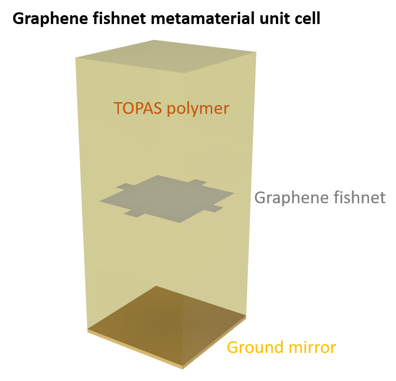
First, the structure and simulation geometry are defined. The structure includes a dielectric substrate with two dielectric patterned layers.

For normal incidence, we can use periodic boundary conditions along the x and y directions. More generally, we need to use Bloch boundary conditions as will be illustrated below. We can also use Bloch boundaries with zero Bloch vector for normal incidence, but a simulation with Bloch boundaries uses complex fields and is twice more computationally expensive than a simulation with periodic boundaries, while the results for bloch_vec = 0 are equivalent.

Web Help Content Version: SOLIDWORKS 2021 SP05 To disable Web help from within SOLIDWORKS and use local help instead, click Help > Use SOLIDWORKS Web Help. To report problems encountered with the Web help interface and search, contact your local support representative. To provide feedback on individual help topics, use the “Feedback on this topic” link on the individual topic page.

We still used a P-polarized source (pol_angle = 0 in the source defition), but now we also get nonzero polarization = "s" amplitudes in the data. This is because the input polarization is at an angle with respect to the x-axis, and is not preserved by the translational invariance along y. Similarly, now there is a nonzero Ey field component in the recorded near fields.

To study a diffraction grating under an angled illumination, we need to use Bloch boundary conditions along the x and y directions that match the incoming wave. The Bloch vector can be automatically computed based on the plane wave parameters, as shown below.

Tidy3D uses a near field to far field transformation specialized to periodic structures to compute the grating efficiency and its accuracy is verified through a comparison with the semi-analytical rigorous coupled wave analysis (RCWA) approach using the open-source library grcwa.

Along z, a perfectly matched layer (PML) is applied to mimic an infinite domain. Because the diffraction grating introduces waves propagating at various angles, including steep angles with respect to the PML boundary, we use more layers than the default value to minimize spurious reflections at the PMLs.

Since this is essentially a 1D grating along x, we'll plot the power, which is normalized and corresponds to the grating efficiency, as a function of x for order 0 in y. The results are in excellent agreement with each other.

Beammomentcalculator

We can also compare to RCWA results as before. Note that, because we are injecting backwards, we need to add an np.pi to angle_theta in the grcwa computation.

Note that grcwa returns fields in Cartesian coordinates, while Tidy3D returns power amplitudes in the s and p polarization basis. Therefore, we will use some convenience methods to convert grcwa's fields to spherical coordinates before comparing the two solvers.

SOLIDWORKS welcomes your feedback concerning the presentation, accuracy, and thoroughness of the documentation. Use the form below to send your comments and suggestions about this topic directly to our documentation team. The documentation team cannot answer technical support questions. Click here for information about technical support.

In this example, we compute the grating efficiency of a multilevel diffraction grating whose design is inspired by M. Oliva, T. Harzendorf, D. Michaelis, U. D. Zeitner, and A. TÃ¼nnermann, "Multilevel blazed gratings in resonance domain: an alternative to the classical fabrication approach," Opt. Express 19, 14735-14745 (2011), DOI: 10.1364/OE.19.014735.

Grating structures are ubiquitous in optics and photonics. In another case study, we investigated the possibility of using a grating structure as a biosensor.

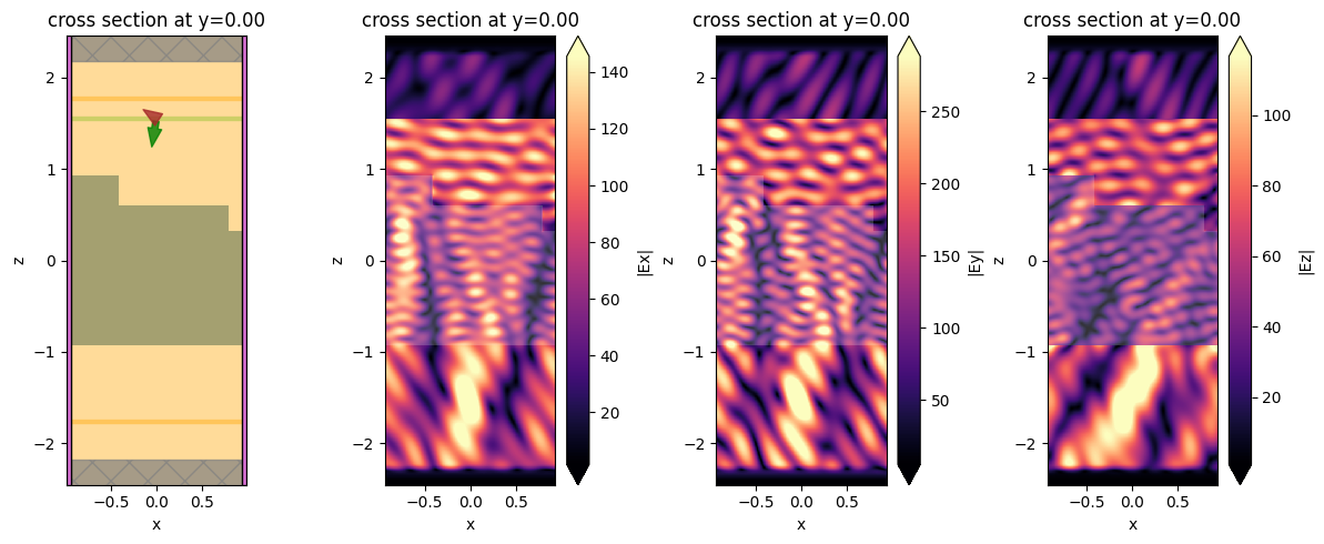
Plot the frequency-domain electric field components at the center frequency along an xz cut of the domain. The y component is zero everywhere because the wave is entirely x-polarized.

Beam calculatorwith solutions

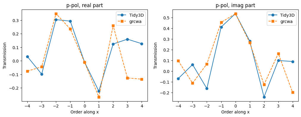
We can also compare the transmitted complex power amplitude for each order and each polarization to those obtained via the grcwa package. The power amplitudes are complex and provide information about the phase difference among different orders.

Beam calculatorapp

If you are new to the finite-difference time-domain (FDTD) method, we highly recommend going through our FDTD101 tutorials.

Enter your email address below to receive the presentation slides. In the future, weâll share you very few emails when we have new tutorial release, development updates, valuable toolkits and technical guidance . You can unsubscribe at any time by clicking the link at the bottom of every email. Weâll never share your information.

If the illumination is such that the angle is non-zero along y, a slightly special treatment is required in that we cannot set the simulation size to zero in that direction anymore. Instead we should define the simulation length to be a small finite value, and set the mesh step in that direction to the same value.