Microscope Objective Lenses for Industry - objective lenses of microscope

 2024-11-25 13:15:01

Dear Simon, Thank you for your interest in my blog. The above formula is written for beams in vacua or air for simplicity. But the formula still holds if you read k as the wave number in a material, that is, if you use n*k instead of k, where n is the refractive index of the material. In COMSOL, the Gaussian beam settings in the background field feature in the Wave Optics module are set for the vacuum by default, i.e., the wave number is set to be “ewfd.k0”. But you can change it to “ewfd.k” for more general cases. COMSOL will automatically take care of the local “k” depending on where you have different materials in your domain. There is a tricky thing you have to keep in mind in this situation: You have to know the waist position wherever it is positioned. If a Gaussian beam is incident from air to glass and makes a focus in the glass, the waist position will be different from the case where the material doesn’t exist (See Applied Optics, Vol. 27, No. 9, p.1834-1839 (1988) ). You have to calculate the focus position first, and then enter the focus position in COMSOL. Best regards, Yosuke

Dear Yosuke, Is the background method applicable to the case of an interface? Suppose the beam is incident from air to glass, is this formular still valid? If not, how to implement the correct one? Thank you Best regards Simon

Dear Daniel, Thank you for reading this blog. When we assumed time-harmonic waves to derive the Helmholtz equation from the time-dependent wave equation, we factored out exp(i*omega*t). Remembering this process, we get a time-dependent wave by putting the factor back, i.e., by replacing exp(-ik*x) with exp(i*(omega*t -k*x)) in the formula in this blog. This is implemented in second_harmonic_generation.mph in our Application Libraries under Wave Optics Module > Nonlinear Optics. I hope this helps! Best regards, Yosuke

Plots showing the electric field norm of paraxial Gaussian beams with different waist radii. Note that the variable name for the background field is ewfd.Ebz.

Dear Jana, Thank you for reading this blog. There are some limitations for the built-in Gaussian beam feature. 1. You can only propagate it along the x or y or z axis. Due to this limitation, you will have to rotate your material in order to simulate a beam at an angle. 2. The focus position needs to be known a priori. This is a little bit tricky to explain but you need to know the focus position inside your material and enter the position in “Focal plane along the axis” section because COMSOL won’t automatically calculate the focus position shift if you only know the field outside your material. Because of the convergence of a Gaussian beam, there will be a refraction at a material interface, which causes the focus shift. For more details about the Gaussian beam focus shift at interfaces, please refer to this paper: Shojiro Nemoto, Applied Optics, Vol. 27, No. 9 (1988). If you would like a more flexible way, you can define a paraxial Gaussian beam in Definition and also define a coordinate transfer. Please send support@comsol.com a question on this method since it’s a little bit difficult to explain here. Best regards, Yosuke

Dear Jana, That was a typo. Correct: y2 = x*sin(theta)+y*cos(theta) Other than that, if you have more questions on this particular one, please send your question to support@comsol.com with your model. That’d be more effective. Best regards, Yosuke

ND filters come in many different strengths. Depending on the manufacturer, these strengths may be notated in one of three ways: stops, optical density, or ND factor. Stops (sometimes referred to as exposure value) are fairly straightforward in that they tell you exactly how many stops your exposure will be adjusted by. Optical density is essentially 0.3 x the exposure value. This is the least common labeling system on the market. The ND factor is often listed as ND2, ND4, ND8, and so on. These numbers refer to the amount by which the light is reduced, ie. ND2 halves the light while ND4 reduces the light to one quarter. The chart below shows the translation between the three labeling systems.

The original idea of the paraxial Gaussian beam starts with approximating the scalar Helmholtz equation by factoring out the propagating factor and leaving the slowly varying function, i.e., E_z(x,y) = A(x,y)e^{-ikx}, where the propagation axis is in x and A(x,y) is the slowly varying function. This will yield an identity

Dear Yosuke, As you know the gaussian beam source that I asked you about I used it in 3D structure and was represented in my model by analytic functon with the next formula: E(x,y,z)= E0*w0/w(x)*exp(-(y^2+z^2)/w(x)^2)*exp(-i*(k*x-eta(x)+k*(y^2+z^2)/(2*R(x)))) And I wrote the component of electric field in propagation direction as following: (j*d(E(x,y,z),z)/emw.k0) where (z) is the polarization direction and I used it to overcome the paraxial approximation problem if you rememer, but I get this error: { Error in user-defined function. – Function: dE_dE__z__internalArgument Failed to evaluate variable. – Variable: comp1.emw.Ebx – Defined as: exp(i*phase)*(!(comp1.isScalingSystemDomain)*(comp1.es.Ex+((j*d((unit_V_cf*E(x/unit_m_cf,y/unit_m_cf,z/unit_m_cf))/unit_m_cf,z))/comp1.emw.k0))) Failed to evaluate expression. – Expression: comp1.emw.Ebx Failed to evaluate operator. – Operator: mean – Geometry: geom1 } Could you tell me the problem here? Thanks

laguerre-gaussianbeam

I am trying to study the optical characteristics of gold nano-particle (radius = 6nm) on a wavelength spectrum extended from 400 nm to 500 nm, and I do not know how I can determine the beam radius waist (w0) value. I think it will be less than wavelength and this will not match with the paraxial approximation for Maxwell equation that used in the suggested gaussian beam in your blog.

Because they can be focused to the smallest spot size of all electromagnetic beams, Gaussian beams can deliver the highest resolution for imaging, as well as the highest power density for a fixed incident power, which can be important in fields such as material processing. These qualities are why lasers are such attractive light sources. To obtain the tightest possible focus, most commercial lasers are designed to operate in the lowest transverse mode, called the Gaussian beam.

By providing your email address, you consent to receive emails from COMSOL AB and its affiliates about the COMSOL Blog, and agree that COMSOL may process your information according to its Privacy Policy. This consent may be withdrawn.

Besselbeam

The paraxial Gaussian beam formula is an approximation to the Helmholtz equation derived from Maxwell’s equations. This is the first important element to note, while the other portions of our discussion will focus on how the formula is derived and what types of assumptions are made from it.

Dear Yasmien, The solution is one of the valid methods for both 3D and 2D. Mesh refinement works for increasing the accuracy of finite element solutions. If you use a loosely focused Gaussian beam, yes, your paraxial Gaussian beam in your finite element model will become closer to the closed-form paraxial Gaussian beam. But if you use a very small waist size in the paraxial Gaussian beam formula, mesh refinement will not work to improve the error coming from the paraxial approximation. It doesn’t change the scalar paraxial approximation nature. The technique used in the model you referred to is actually a remedy to the fact that the Gaussian beam starts to show its vectorial nature when it’s tightly focused, which is negligibly small when the focusing is not tight where the scalar paraxial Gaussian beam formula is valid. Best regards, Yosuke

Thanks Yosuke, When I write an expession for x2, as you mentioned above, it shows Syntax error in expression – Expression: x*cos(theta) – y*sin(theta) – Subexpression: – y*sin(the – Position: 14 Error in automatic sequence generation. Is last expression for y2 right, because in both parts there is x? Can I define x and y are equal to 1? Regards Jana

COMSOLGaussian beam

Gaussian beamcalculator

Dear Yosuke, Thank you for this clear and informative demonstration of the paraxial beam functionality in COMSOL! At the moment I am working on in bulk laser material processing of sapphire where I need to define an Gaussian beam entering the material and focusing in the bulk. Since this process is time dependent ( we want to study the behavior ), I am looking for a time dependent description of the Gaussian beam to take into account the varying pulse energy. I noticed that the Gaussian beam is only available in the frequency domain, what do I need to know and model to study this in a time dependent study? Daniel

Note: It is important to be clear about which quantities are given and which ones are being calculated. To specify a paraxial Gaussian beam, either the waist radius w_0 or the far-field divergence angle \theta must be given. These two quantities are dependent on each other through the approximate divergence angle equation. All other quantities and functions are derived from and defined by these quantities.

This factorization is reasonable for a wave in a laser cavity propagating along the optical axis. The next assumption is that |\partial^2 A/ \partial x^2| \ll |2k \partial A/\partial x|, which means that the envelope of the propagating wave is slow along the optical axis, and |\partial^2 A/ \partial x^2| \ll |\partial^2 A/ \partial y^2|, which means that the variation of the wave in the optical axis is slower than that in the transverse axis. These assumptions derive an approximation to the Helmholtz equation, which is called the paraxial Helmholtz equation, i.e.,

Dear Yasmien, That means there is no purely linearly polarized beam for non-paraxial Gaussian beams. There is a reference in the pdf document for the nanorods model, M. Lax, W.H. Louisell, and W. B. McKnight, “From Maxwell to paraxial wave optics”, Physical Review A, vol. 11, no. 4, pp. 1365-1370 (1975). You don’t want to simulate what really doesn’t exist, do you? If your beam is really a tightly focused beam, it has a propagation component inevitably. So you have to add it no matter how it’s a different component than your preferred plane to which you want to believe it’s polarized. Best regards, Yosuke

There are additional approaches available for simulating the Gaussian beam in a more rigorous manner, allowing you to push through the limit of the smallest spot size. We will discuss this topic in a future blog post. Stay tuned!

The results shown above clearly indicate that the paraxial Gaussian beam formula starts failing to be consistent with the Helmholtz equation as it’s focused more tightly. Quantitatively, the plot below may illustrate the trend more clearly. Here, the relative L2 error is defined by \left ( \int_\Omega |E_{\rm sc}|^2dxdy / \int_\Omega |E_{\rm bg}|^2dxdy \right )^{0.5}, where \Omega stands for the computational domain, which is compared to the mesh size. As this plot suggests, we can’t expect that the paraxial Gaussian beam formula for spot sizes near or smaller than the wavelength is representative of what really happens in experiments or the behavior of real electromagnetic Gaussian beams. In the settings of the paraxial Gaussian beam formula in COMSOL Multiphysics, the default waist radius is ten times the wavelength, which is safe enough to be consistent with the Helmholtz equation. It is, however, not a “cut-off” number, as the approximation assumption is continuous. It’s up to you to decide when you need to be cautious in your use of this approximate formula.

Mathematics of vectorialgaussianbeams

Dear Yosuke, Thanks for your kind reply, it is very helpful, and yes I want to focus the beam to the size of the nano-particle with 6 nm radius, but I have 2 questions if you kindly allow: 1) I realized that you determine the waist radii depending on the wavelength only, Do you divide it by (pi)?, ignoring the particle radius. The second part of my question is should I depend on one factor only in determining w0 that is wavelength only? 2) When you write that 4 um is the proper w0, Do you mean that I can use this value for the whole previous wavelength spectrum? I mean is it constant? Best regards

Thanks Yosuke for such an interesting and clear post. The model I am currently working on includes a Gaussian beam focused by a high NA objective lens. Clearly, this is too tightly focused for the paraxial approximation to hold, and I encountered the problems you have described above. However, searching around the web I wasn’t able to find out so far anyone coming up with a workaround to these limitations. More in general, is there a way to simulate in COMSOL the point spread function of a high NA lens? You can imagine I am now really looking forward to the follow-up post you promised describing the solutions! I am wondering, are you planning to publish this any soon? Would you be able meanwhile to point to me some useful information on this matter? With kind regards, Attilio

Gaussian beamOptics CVI laser Optics idex Optics photonics

I read your kind answer carefully and understood it. I am really thankful to this discussion with you because I do learn from it, so excuse me in this extra question;

Thanks for your kind reply, it is very helpful, and yes I want to focus the beam to the size of the nano-particle with 6 nm radius, but I have 2 questions if you kindly allow:

Dear Yasmien, Thank you very much for reading my blog and for your interest. Do you have to focus your beam to the size of the nano-particle? The beam waist size is determined depending on how much you have to focus. For that wavelength range, the least possible waist radii are as large as 127 nm to 159 nm, though. And for these numbers, the paraxial formula will not give you an accurate result. If a slow (gently focusing) beam works for your characterization, the waist radius of 4 um or larger would work and our Gaussian beam background feature gives you a correct result.

Thanks for your clarification and I got the idea in using mesh. The explanation of the reason of existence an electric field component in the propagation direction is still unclear to me, I am sorry I did not understand it well. Also, why do we represent this component by differentiating the gaussian beam field according to the polarization direction?

The Gaussian beam is recognized as one of the most useful light sources. To describe the Gaussian beam, there is a mathematical formula called the paraxial Gaussian beam formula. Today, we’ll learn about this formula, including its limitations, by using the Electromagnetic Waves, Frequency Domain interface in the COMSOL Multiphysics® software. We’ll also provide further detail into a potential cause of error when utilizing this formula. In a later blog post, we’ll provide solutions to the limitations discussed here.

Dear Attilio, Thank you for reading my blog post and for your comment. We will publish a follow-up blog post with rigorous solutions in a few months. In the meantime, you may want to check out this reference: P. Varga et al., “The Gaussian wave solution of Maxwell’s equations and the validity of scalar wave approximation”, Optics Communications, 152 (1998) 108-118. In this paper, the authors give an exact formula for a nonparaxial Gaussian wave. Best regards, Yosuke

Plots showing the electric field norm of the scattered field. Note that the variable name for the scattered field is ewfd.relEz. Also note that the numerical error is contained in this error field as well as the formula’s error.

Dear Yasmien, 1) You can not focus a beam to an infinitely small size. Yes, the number I gave you is lambda/pi. I have no proof for this but it is what I know as the smallest possible spot size for a wavelength no matter what your particle size is. The wavelength is not the determining factor of w0. The minimum beam waist radius is determined by how the laser beam has originally been generated inside a laser cavity. You can’t change it. You can focus the beam by a focusing lens but you can only worsen it or at most you can keep it as it is depending on the lens quality. So when you simulate a focusing laser beam, you should have the specification of the laser beam. 2) I gave w0 = 10 lambda. If your wavelength is 400 nm, 10×400 nm = 4 um is the waist radius for which the paraxial Gaussian beam is a good approximation. For 500 nm, it’d be 5 um. Best regards, Yosuke

When I write an expession for x2, as you mentioned above, it shows Syntax error in expression – Expression: x*cos(theta) – y*sin(theta) – Subexpression: – y*sin(the – Position: 14 Error in automatic sequence generation.

In the above plot, we saw the relationship between the waist size and the accuracy of the paraxial approximation. Now we can check the assumptions that were discussed earlier. One of the assumptions to derive the paraxial Helmholtz equation is that the envelope function varies relatively slowly in the propagation axis, i.e., |\partial^2 A/ \partial x^2| \ll |2k \partial A/\partial x|. Let’s check this condition on the x-axis. To that end, we can calculate a quantity representing the paraxiality. As the paraxial Helmholtz equation is a complex equation, let’s take a look at the real part of this quantity, {\rm abs} \left ( {\rm real} \left ( (\partial^2 A/ \partial x^2) / (2ik \partial A/\partial x) \right ) \right ).

Editor’s note, 7/2/18: The follow-up blog post, “The Nonparaxial Gaussian Beam Formula for Simulating Wave Optics”, is now live.

You can imagine I am now really looking forward to the follow-up post you promised describing the solutions! I am wondering, are you planning to publish this any soon? Would you be able meanwhile to point to me some useful information on this matter?

The above equation is the scattered field formulation, where COMSOL Multiphysics solves for the scattered field. This formulation can be viewed as a scattering problem with a scattering potential, which appears in the right-hand side. It is easy to understand that the scattered field will be zero if the background field satisfies the Helmholtz equation (under an approximate Sommerfeld radiation condition, such as an absorbing boundary condition) because the right-hand side is zero, aside from the numerical errors. If the background field doesn’t satisfy the Helmholtz equation, the right-hand side may leave some nonzero value, in which case the scattered field may be nonzero. This field can be regarded as an error of the background field. In other words, under certain conditions, you can qualify and quantify exactly how and by how much your background field satisfies the Helmholtz equation. Let’s now take a look at the scattered field for the example shown in the previous simulations.

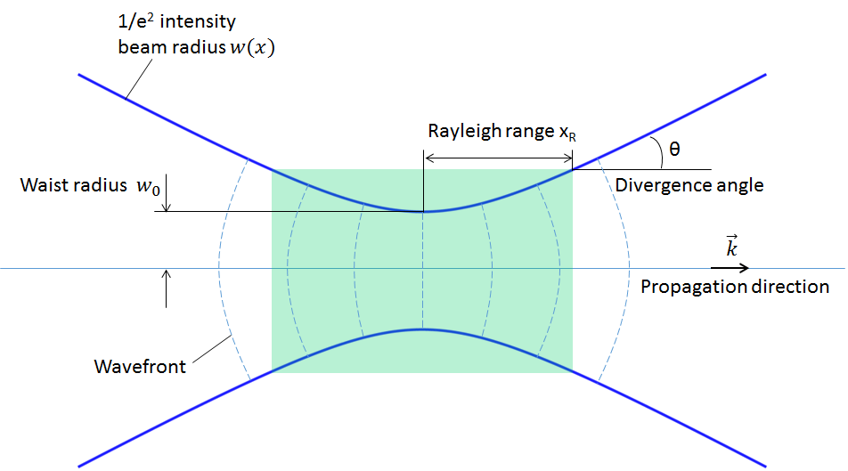
Here, x_R is referred to as the Rayleigh range. Outside of the Rayleigh range, the Gaussian beam size becomes proportional to the distance from the focal point and the 1/e^2 intensity position diverges at an approximate divergence angle of \theta = \lambda/(\pi w_0).

For a rotated one at an angle theta, please replace x and y in the above expression with x2 and y2 and define x2 = x*cos(theta) – y*sin(theta) y2 = x*sin(theta) + x*cos(theta)

The following plot is the result of the calculation as a function of x normalized by the wavelength. (You can type it in the plot settings by using the derivative operand like d(d(A,x),x) and d(A,x), and so on.) We can see that the paraxiality condition breaks down as the waist size gets close to the wavelength. This plot indicates that the beam envelope is no longer a slowly varying one around the focus as the beam becomes fast. A different approach for seeing the same trend is shown in our Suggested Reading section.

The paraxial Gaussian beam option will be available if the scattered field formulation is chosen, as illustrated in the screenshot below. By using this feature, you can use the paraxial Gaussian beam formula in COMSOL Multiphysics without having to type out the relatively complicated formula. Instead, you simply need to specify the waist radius, focus position, polarization, and the wave number.

In the scattered field formulation, the total field E_{\rm total} is linearly decomposed into the background field E_{\rm bg} and the scattered field E_{\rm sc} as E_{\rm total} = E_{\rm bg} + E_{\rm sc}. Since the total field must satisfy the Helmholtz equation, it follows that (\nabla^2 + k^2 )E_{\rm total} = 0, where \nabla^2 is the Laplace operator. This is the full field formulation, where COMSOL Multiphysics solves for the total field. On the other hand, this formulation can be rewritten in the form of an inhomogeneous Helmholtz equation as

One of the COMSOL modes named “Nanorods” with application library path: Wave_Optics_Module/Optical_Scattering/ nanorods. In the “Model Definition” section at page 1 of this model, the author determined that the rods have dimensions less than wavelength, as my case, and as I understand he overcame the problem of Gaussian beam is an approximation solution by the following sentence and I will write it as it was reminded ” For tightly focused beams you also need to include an electric field component in the propagation direction”.

When searching for ND filters, we believe that labeling with the number of stops is the easiest way to understand exactly how they will affect your images. Our Kolari Pro ND Filters come in a wide range of strengths from 1-stop to 20-stops, and our Kolari Pro VND is available in 2-5 stops and 6-9 stops options.

Hi, I am rather new to Comsol. Thanks for this good explanation of Gaussian beam. I have a question: What should I change/add to incident a Gaussian beam at interface with some degree of angle if the scattered field formulation is chosen (as you have shown in window above)?

Could you tell me the proper choice for the value of w0 and how can I use the gaussian beam formula as a background source in my case.

Dear Yasmien, Can you please go through our technical support, support@comsol.com? We need to see your model to solve your problem. Thank you. Yosuke

Dear Yosuke Mizuyama Very interested topic. I have one question, please. Why lambda is equal to 500nm and used in COMSOL as the default value for the calculation of frequency (f=c_const/500[nm])?

As you know the gaussian beam source that I asked you about I used it in 3D structure and was represented in my model by analytic functon with the next formula: E(x,y,z)= E0*w0/w(x)*exp(-(y^2+z^2)/w(x)^2)*exp(-i*(k*x-eta(x)+k*(y^2+z^2)/(2*R(x))))

Dear Yosuke Mizuyama： Thanks Yosuke for such an interesting and clear post.My current work is a single crystal fiber laser, and I encountered the problem you described above while simulating the propagation of light in the pump!I am here to ask you what method can I use to simulate the propagation of a Gaussian beam (W0 =0.147mm) in a rod with a diameter of 1mm and display the light intensity distribution!I used the ray tracing module, but the results are too poor. Can you tell me how to implement my simulation?Thank you very much!

Today’s blog post has covered the fundamentals related to the paraxial Gaussian beam formula. Understanding how to effectively utilize this useful formulation requires knowledge of its limitation as well as how to determine its accuracy, both of which are elements that we have highlighted here.

{ Error in user-defined function. – Function: dE_dE__z__internalArgument Failed to evaluate variable. – Variable: comp1.emw.Ebx – Defined as: exp(i*phase)*(!(comp1.isScalingSystemDomain)*(comp1.es.Ex+((j*d((unit_V_cf*E(x/unit_m_cf,y/unit_m_cf,z/unit_m_cf))/unit_m_cf,z))/comp1.emw.k0))) Failed to evaluate expression. – Expression: comp1.emw.Ebx Failed to evaluate operator. – Operator: mean – Geometry: geom1 }

And I wrote the component of electric field in propagation direction as following: (j*d(E(x,y,z),z)/emw.k0) where (z) is the polarization direction and I used it to overcome the paraxial approximation problem if you rememer, but I get this error:

Laguerre-Gaussian mode

Dear Yosuke, Thanks for your clarification and I got the idea in using mesh. The explanation of the reason of existence an electric field component in the propagation direction is still unclear to me, I am sorry I did not understand it well. Also, why do we represent this component by differentiating the gaussian beam field according to the polarization direction? Could you recommend a source for reading?

Away from the previous question, do you think that decreasing the mesh size would increase the accuracy of gaussian beams in small structures?

Dear Yosuke, I read your kind answer carefully and understood it. I am really thankful to this discussion with you because I do learn from it, so excuse me in this extra question; One of the COMSOL modes named “Nanorods” with application library path: Wave_Optics_Module/Optical_Scattering/ nanorods. In the “Model Definition” section at page 1 of this model, the author determined that the rods have dimensions less than wavelength, as my case, and as I understand he overcame the problem of Gaussian beam is an approximation solution by the following sentence and I will write it as it was reminded ” For tightly focused beams you also need to include an electric field component in the propagation direction”. My question: is this solution appropriate in 3D or in 2D structures only? Away from the previous question, do you think that decreasing the mesh size would increase the accuracy of gaussian beams in small structures? I will wait your kind answer and really thank you in advance.

Dear Yosuke, Thank you so much for this reliable blog. I have a question about one of limitations of paraxial gaussian beam. I am trying to study the optical characteristics of gold nano-particle (radius = 6nm) on a wavelength spectrum extended from 400 nm to 500 nm, and I do not know how I can determine the beam radius waist (w0) value. I think it will be less than wavelength and this will not match with the paraxial approximation for Maxwell equation that used in the suggested gaussian beam in your blog. Could you tell me the proper choice for the value of w0 and how can I use the gaussian beam formula as a background source in my case. Thanks in advance

1) I realized that you determine the waist radii depending on the wavelength only, Do you divide it by (pi)?, ignoring the particle radius. The second part of my question is should I depend on one factor only in determining w0 that is wavelength only?

The special solution to this paraxial Helmholtz equation gives the paraxial Gaussian beam formula. For a given waist radius w_0 at the focus point, the slowly varying function is given by

Thanks Yosuke, Could you please guide me how I can write an expression for a gaussian beam (in 2D) propagating in x-direction while the polarization in y-direction? And, also how I can define a coordinate transfer in expression for an incident angle of the beam? Regards, Salman

Note: The term “Gaussian beam” can sometimes be used to describe a beam with a “Gaussian profile” or “Gaussian distribution”. When we use the term “Gaussian beam” here, it always means a “focusing” or “propagating” Gaussian beam, which includes the amplitude and the phase.

As such, it would be reasonable to want to simulate a Gaussian beam with the smallest spot size. There is a formula that predicts real Gaussian beams in experiments very well and is convenient to apply in simulation studies. However, there is a limitation attributed to using this formula. The limitation appears when you are trying to describe a Gaussian beam with a spot size near its wavelength. In other words, the formula becomes less accurate when trying to observe the most beneficial feature of the Gaussian beam in simulation. In a future blog post, we will discuss ways to simulate Gaussian beams more accurately; for the remainder of this post, we will focus exclusively on the paraxial Gaussian beam.

高斯光束

Since ND filters are used to reduce the amount of light in a scene, each stop is always halving the amount of light. The larger the stop number, the more light the filter blocks out.

Dear Jana, Here’s the expression: Ex = 0 Ey = sqrt(w0/w(x))*exp(-y^2/w(x)^2)*exp(-i*k*x-i*k*y^2/(2*R(x))-eta(x)) Ez = 0 w0 = given waist radius, k = 2*pi/lambda w(x) = w0*sqrt(1+(x/xR)^2) xR = pi*w0^2/lambda R(x) = x+xR^2/x eta(x) = atan(x/xR)/2 For a rotated one at an angle theta, please replace x and y in the above expression with x2 and y2 and define x2 = x*cos(theta) – y*sin(theta) y2 = x*sin(theta) + x*cos(theta) Best regards, Yosuke

where w(x), R(x), and \eta(x) are the beam radius as a function of x, the radius of curvature of the wavefront, and the Gouy phase, respectively. The following definitions apply: w(x) = w_0\sqrt{1+\left ( \frac{x}{x_R} \right )^2 }, R(x) = x +\frac{x_R^2}{x}, \eta(x) = \frac 12 {\rm atan} \left ( \frac{x}{x_R} \right ), and x_R = \frac{\pi w_0^2}{\lambda}.

You can see how as the filter strength increases, the exposure time is doubled sequentially to compensate for the loss of light. When the light is cut in half, you need to double the shutter speed to maintain the same exposure. Add another ND stop, double the shutter speed again.

Thank you for this clear and informative demonstration of the paraxial beam functionality in COMSOL! At the moment I am working on in bulk laser material processing of sapphire where I need to define an Gaussian beam entering the material and focusing in the bulk. Since this process is time dependent ( we want to study the behavior ), I am looking for a time dependent description of the Gaussian beam to take into account the varying pulse energy. I noticed that the Gaussian beam is only available in the frequency domain, what do I need to know and model to study this in a time dependent study?

Because the laser beam is an electromagnetic beam, it satisfies the Maxwell equations. The time-harmonic assumption (the wave oscillates at a single frequency in time) changes the Maxwell equations to the frequency domain from the time domain, resulting in the monochromatic (single wavelength) Helmholtz equation. Assuming a certain polarization, it further reduces to a scalar Helmholtz equation, which is written in 2D for the out-of-plane electric field for simplicity:

Where this gets tricky is knowing the mathematical order of operations for the different stops. For example, a 1-stop ND will reduce the light by 50% and a 5-stop will cut the light in half five times in a row. If you have a 1-second exposure without a filter and then put on a 1-stop ND filter, you have effectively halved the amount of light coming into your camera. In order to balance out the exposure, you’ll have to increase your shutter speed by doubling it. Now, your 1-second exposure becomes 2 seconds.

2) When you write that 4 um is the proper w0, Do you mean that I can use this value for the whole previous wavelength spectrum? I mean is it constant?

Dear Yosuke Mizuyama Very interested topic. I have one question, please. Why lambda is equal to 500nm and used in COMSOL as the default value for the calculation of frequency (f=c_const/500[nm])?

Dear Yasmien, Can you please go through our technical support, support@comsol.com? We need to see your model to solve your problem. Thank you. Yosuke

In COMSOL Multiphysics, the paraxial Gaussian beam formula is included as a built-in background field in the Electromagnetic Waves, Frequency Domain interface in the RF and Wave Optics modules. The interface features a formulation option for solving electromagnetic scattering problems, which are the Full field and the Scattered field formulations.