In the lexicon of photography, the F/# denotes the “speed” of the optics, with fast lenses having low F/#. The aperture control on a camera changes the F/# by using an iris diaphragm to change D.

In introducing the concept of G, we required that the optical system in Fig.13 had no internal limiting apertures.This meant that G was determined by the source area and input acceptance angle of the optical system. In this case, for more total flux through the system from a source of fixed size and radiance, all that is needed is to increase G. This is equivalent to decreasing condenser F/# as previously discussed.

Before hyperspectral imaging devices were readily available, researchers wishing to quantify effects based on colour information have used multispectral imaging, or hyperspectral, point-source devices (such as spectroradiometers which do not produce a spatial image) to acquire colour data. Hyperspectral devices do not in general provide a point-and-click measurement. Instead, much onus is on the user to develop the capture process. Once acquired, the resulting large numerical datasets must be analysed in order to provide useful information. A sensible and simple way into such large datasets is to consider only a small number of positions in the wavelength range, looking at changes across conditions at predetermined key points in the spectrum. Using this approach, we can also counter the effects of relative light changes by considering ratios of data values. This involves the combination of two or more wavelengths, commonly known as ‘indices’.

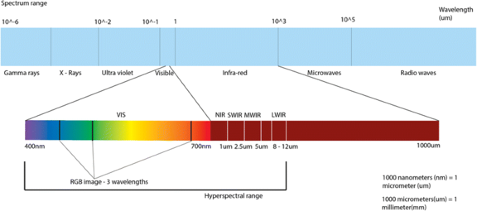
The range of light captured in a hyperspectral system can also vary. The colour visible to the human eye is a small range on the electromagnetic spectrum, ranging from 400 to 700 nm (Fig. 1). The section of the spectrum that is typically used for hyperspectral imaging of plants ranges from ultraviolet (UV) (starting at ~ 250 nm) up to short-wave infrared (SWIR, ~ 2500 nm). Cameras usually capture a certain sub-range, such as the visible and near infrared range (VIS–NIR, 400–1300 nm) or the SWIR (1300–2500 nm) or UV (250–400 nm) with the ranges being combined in some sensors to increase the coverage of the spectrum.

Concave spherical mirrors are also used to collect and focus light. We use them for our Fiber Illuminators. The focal length of a lens can vary with wavelength due to chromatic aberration, while mirror systems are truly wideband in application. The concepts of F/# and numerical aperture also apply to mirrors. When elliptical reflectors are used, as in our PhotoMax™ Lamp Housings, F/# is used to describe the ratio of the reflector aperture to the distance between that aperture and the focus outside the ellipse.

Sims DA, Gamon JA. Relationships between leaf pigment content and spectral reflectance across a wide range of species, leaf structures and developmental stages. Remote Sens Environ. 2002;81:337–54.

Barnes JD, Balaguer L, Manrique E, Elvira S, Davison AW. A reappraisal of the use of DMSO for the extraction and determination of chlorophylls a and b in lichens and higher plants. Environ Exp Bot. 1992;32:85–100.

Kersting K, Xu Z, Wahabzada M, Bauckhage C, Thurau C, Roemer C, et al. Pre-symptomatic prediction of plant drought stress using dirichlet-aggregation regression on hyperspectral images. AAAI [Internet]. 2012 [cited 2015 Nov 3]. https://www.aaai.org/ocs/index.php/AAAI/AAAI12/paper/view/4932.

Behmann J, Steinrücken J, Plümer L. Detection of early plant stress responses in hyperspectral images. ISPRS J Photogramm Remote Sens. 2014;93:98–111.

Our Off-Axis Paraboloidal Reflectors are a circular segment from one side of a full paraboloid. The focal point is off the mechanical axis, giving full access to the reflector focus area (Figure 8). There are no shadowing problems if you place a detector or source at the focus. Note that these mirrors do introduce significant aberrations for extended sources.

Römer C, Wahabzada M, Ballvora A, Rossini M, Panigada C, Behmann J, et al. Early drought stress detection in cereals: simplex volume maximisation for hyperspectral image analysis. Funct Plant Biol. 2012;39:878–90.

F number napdf

Satterwhite MB, Henley JP. Hyperspectral signatures (400 to 2500 nm) of vegetation, minerals, soils, rocks, and cultural features: laboratory and field measurements 1990.

Spectral angle mapper (SAM) approaches match the pixel spectra to reference spectra to classify the pixels by calculating the angle between the spectra which are treated as n-dimensional vectors in space [2]. This technique has been widely used with moderate success to classify hyperspectral data, including plant diseases. Yuhas studied the severity of Fusarium head blight disease for wheat before harvesting. The hyperspectral data was in the range 400–1000 nm with a spectral resolution of 2.5 nm. SAM was used to detect the amount of disease with a classification accuracy of 87%. Two experiments with wheat plants were carried out, one in a glasshouse and one in field. The plants were imaged over their developmental stages from inoculated to established infection. Yuhas determined that just after infection, the healthy and infected plants were not distinguishable because the infection had not yet established. However, when the hyperspectral data were examined during the ripening stage, the wheat pigment composition changes, and the healthy plants then appear as diseased plants [39].

Along with detecting and classifying disease, we may wish to record the effective amount of disease, or its severity. This approach does run into some particular challenges. The amount of leaf damage and coverage from the disease can affect the accuracy of the leaves being classified as healthy or diseased. Extreme disease damage can affect the appearance of leaves so detrimentally that they may not be counted as plant material at all. Still, there are a number of methods for estimating severity, and we present a selection of approaches below.

Prior to analysis, the hyperspectral data needs to be calibrated to ensure the images produced are adjusted due to the colour of lighting present; the camera software may have this option, but if it does not then the data can be calibrated after it is captured. The lighting is calibrated using a known white balance target, which is imaged by the camera system. This target will reflect a known percentage of light over the spectrum, for example 99% across the entire working spectrum of the camera. Non-uniformity of illumination can be corrected for by dividing the observed data by the captured white balance data [49]. Additionally, the system must be corrected for electrical noise present from the sensor in the absence of light (called dark current). This is usually carried out by taking an image with the camera in the absence of any light, and using the resultant low-level noise readings to adjust future measures.

The ultraviolet transmittance of condensers and other optical elements is important when trying to conserve the limited ultraviolet components from our sources. The ultraviolet transmittance of *“quartz” or “fused silica” is very dependent on the origin of the material and on the cumulative exposure to short wavelength radiation (solarization). Our condensers are made from selected UV grade synthetic silica for the best ultraviolet transmittance.

Fig. 11 shows the same lens at three different distances from a source. According to the definition of Fig.1, the F/# of the lens is f/D, but obviously the light collected by the same lens differs significantly for each position. The description should include the F/# for collection and the F/# for imaging.

Another commonly-used approach is to detect changes in the sudden increase in reflectance at the red/near-infrared border. This ‘red edge’ position is a narrow section in the electromagnetic spectrum (690–740 nm) where the visible spectrum ends and the near infrared starts (Fig. 2). This section has a large change in spectral response (derivative),for green plant material, since chlorophyll strongly absorbs wavelengths up to around 700 nm, and hence the material has low reflectance in this range, but it is strongly reflecting the infrared (from about 720 nm). Cho [24] describes a number of different algorithms that extract or detect the red edge. A disease index based on the red edge position has been used to detect powdery mildew in wheat (Blumeria graminis f. sp. Tritici), however it was not as accurate as Partial Least Squares Regression (PLSR), a technique that uses a statistical approach [25]. We will consider some of these statistical approaches further in this review.

Verrelst J, Koetz B, Kneubühler M, Schaepman M. Directional sensitivity analysis of vegetation indices from multi-angular Chris/PROBA data. In: ISPRS commission VII-term symposium [Internet]. 2006 [cited 2015 Nov 3]. p. 677–83. http://www.isprs.org/proceedings/XXXVI/part7/

Other non-deep learning approaches include Yuan [30], using Fishers Linear Discriminant Analysis with remote sensing data to detect yellow rust and powdery mildew for a wheat crop with an overall accuracy of 93% with selected wavelength ranges (531, 570–654, 685–717 nm) that are significant for detecting differences between powdery mildew and yellow rust diseases in these spectral reflectance ranges, resulting from an independent t test.

*Again, an aberration free optical system is assumed. When aberrations are present, tGL becomes an upper limit on achievable flux: φ ≤tGL.

Qin J, Burks TF, Ritenour MA, Bonn WG. Detection of citrus canker using hyperspectral reflectance imaging with spectral information divergence. J Food Eng. 2009;93:183–91.

Moshou D, Bravo C, West J, Wahlen S, McCartney A, Ramon H. Automatic detection of “yellow rust” in wheat using reflectance measurements and neural networks. Comput Electron Agric. 2004;44:173–88.

Cao X, Luo Y, Zhou Y, Fan J, Xu X, West JS, et al. Detection of powdery mildew in two winter wheat plant densities and prediction of grain yield using canopy hyperspectral reflectance. In: Grosch R, editor. PLOS ONE. 2015;10:e0121462.

Figure 1 shows a lens of clear aperture D, collecting light from a source and collimating it. The source is one focal length, f, from the lens. Since most sources radiate at all angles, it is obvious that increasing D or decreasing f allows the lens to capture more radiation.The F-number concept puts these two together to allow a quick comparison of optics.

Classification approaches aim to divide the data into a number of distinct classes. They originate from a family of statistical or machine learning techniques. One such approach is quadratic discriminant analysis (QDA), which classifies by using a covariance matrix, which compares classes. The QDA method was used in a study with Avocado plants, to examine the fungal disease Laurel wilt (Raffaelea lauricola), using plants located both in the field and glasshouse. The QDA classification accuracy was 94% [33]. It is possible of course to use alternative methods at each stage of the analysis pipeline. For example, rather than use QDA, a decision tree approach (a machine learning technique) has been used and reached 95% accuracy [33]. Choosing the correct approach for the data, as well as ensuring sufficient dataset size and quality, is key. Such machine learning approaches represent an increasingly-common set of classification and prediction algorithms. Machine learning approaches train algorithms using a training dataset, with the aim of analysing and predicting results from new, unseen data. Multilayer perceptron’s (MLP) are an example of such a technique. MLP’s are simple networks (called artificial neural networks) that maps input data to an output. This process is based on biological understanding of neuron activation networks where messages are fired between neurons. The input node connects to the output and it is updated using an activation function and weights that can be optimised to produce the correct output (using training data). This algorithm requires prior knowledge (training data) therefore if the ‘disease spectra’ is unknown then this technique will be unsuitable.

Simplex volume maximisation selects spectral signatures that are the furthest away from each other to maximise the volume (for example healthy and diseased signatures). Once the signatures have been selected the remaining signatures are assigned to the class they are similar to

Numerical aperture formula

Mahlein A-K, Steiner U, Hillnhütter C, Dehne H-W, Oerke E-C. Hyperspectral imaging for small-scale analysis of symptoms caused by different sugar beet diseases. Plant Methods. 2012;8:3.

As well as detecting the presence of disease, another avenue of research is to distinguish between different diseases to identify specific pathogens. One such approach is spectral information divergence classification. This method compares the divergence between the observed spectra and a reference spectra (a library of spectra, or average spectra of interest from the data), where the smaller the divergence value then the more similar the spectra are, and if they are larger than a set threshold then they are not classified as the reference spectra [3]. Spectral information divergence was used to detect canker legions on citrus fruit (grapefruits) where the spectral range of the data was 450–930 nm with 92 bands and 5.2 nm spectral resolution. Before analysing the data, a pre-processing step is applied by combining neighbouring pixels to reduce the size by half. Cankerous grapefruits were compared with normal grapefruit and also with grapefruit showing other disease or damage symptoms including: greasy spot, insect damage, melanose, scab and wind scar; this method resulted in 95.2% classification accuracy [38].

The practical limit of F/# for singlet Spherical Lenses depends on the application. For high performance imaging, the limit is about F/4. F/2 - F/1.5 is acceptable for use as a condenser with arc lamps. The lens must be properly shaped and the correct side turned towards the source (our F/1.5 plano convex condensers have much poorer aberration performance if reversed).

Artificial neural network—neural networks with input vector and output vectors (neurons/nodes) with one or multiple hidden layers of nodes, where all of the layers are fully connected with weights and an activation function

Another potential difference between laboratory and field imaging is resolution. For aerial remote sensing data, the spatial resolution is typically in the range of meters per pixel, which means the pixels will usually contain signatures from more than one material [14, 15]. A first step in analysing this data is to consider this multi-material problem, whereby pixels must be considered to contain mixed materials (called ‘mixed pixels’) [16, 17], and a spectral unmixing process must be applied. In other words, a single pixel may contain plant and soil, and algorithms must be used to determine the appropriate mix. In the laboratory, images can typically be taken within centimetres of the plant, and there may be many pixels representing even a single leaf or region of disease. In these cases, unmixing is generally not necessary.

Quadratic discriminant analysis classifies using a covariance matrix where each class has a unique matrix and therefore has different class density probabilities

Huang [35] tries to detect Sclerotinia rot disease in Celery crops by using partial least squares regression (PLSR) with derivatives of first and second order. Partial least squares regression selects a small set of components. This technique is useful when the predictors are collinear/highly correlated, and it will reduce the risk of overfitting the data. The classification accuracy for Partial least squares regression with the raw spectra is 88.92%, PLSR with Savitzky-Golay first derivative is 88.18% and PLRS with second order derivative is 86.38%. The accuracies are similar, with the second order derivative performing slightly worse. Yuan [36] uses PLSR on Fisher’s linear discriminant analysis (FLDA) to detect pest and disease in wheat. It produced a 60% accuracy for aphid damage and a 92% accuracy for Yellow rust disease. In another study, Zhang [37] used FLDA to detect powdery mildew in wheat (using a heavily damaged leaf) with over 90% accuracy.

Yuan L, Huang Y, Loraamm RW, Nie C, Wang J, Zhang J. Spectral analysis of winter wheat leaves for detection and differentiation of diseases and insects. Field Crops Res. 2014;156:199–207.

The larger the N.A., the more flux is collected. In air, the maximum N.A. is 1. Microscope objectives are available with N.A. of 0.95.

One technique in particular which has become popular for early detection of drought stress is simplex volume maximisation (SiVM), which is a data clustering technique [43]. This technique selects spectral signatures that are samples of healthy and stressed plants, and then clusters the data using these classes. When the signatures become similar to a pre-learned sample signature then it is classified as such.

Yuhas RH, Goetz AF, Boardman JW. Discrimination among semi-arid landscape endmembers using the spectral angle mapper (SAM) algorithm. In: Summaries of the third annual JPL airborne geoscience workshop [Internet]. Pasadena, CA: JPL Publication; 1992 [cited 2015 Nov 3]. p. 147–9. http://ntrs.nasa.gov/archive/nasa/casi.ntrs.nasa.gov/19940012238.pdf.

By using this website, you agree to our Terms and Conditions, Your US state privacy rights, Privacy statement and Cookies policy. Your privacy choices/Manage cookies we use in the preference centre.

This ratio does not apply to small asymmetrical sources such as the arcs of our arc lamps. Each source must be examined individually.

Decision tree has a tree structure form and it is has decision nodes and leaf nodes where the decision nodes have two or more branches and the leaf nodes represent the classification. This is supervised and needs training. The decision rules can become complex as the tree depth increases

Invariants are of particular value when designing systems in spectroscopy. Monochromators have acceptance angles, slit heights, and slit widths set to give desired resolution. These define the value of the optical extent G, of the monochromator, and allow comparison of different systems and selection of light source optics. The comparison is no longer simply based on F/# of the monochromator. A low F/# monochromator may have lower optical extent, i.e., less throughput, than a monochromator with higher F/#, but which uses larger slits to give the desired resolution. For example, our 1/8 m and our 1/4 m Monochromators have approximately the same F/# but the 1/4 m has a higher Glim for the same resolution.

Partial least squares regression—using linear regression to find the small set of variables from a large set of predictors by finding the latent variables (covariance of the predictors and variables)

An example of multi layer perceptrons (MLP) is described in Moshou [27], who aimed to detect yellow rust in field-grown wheat using a spectrograph with the range 460–900 nm and a 20 nm spectral resolution. The spectrograph captured the images in the field using a handheld system. Then four significant wavelengths were selected. The first two wavelengths were selected using ‘variable selection’ which involved comparing the wavelengths using stepwise discriminant analysis and using the F-test. The second pair of wavelengths uses the NDVI wavelengths. The neural network used by Moshou is a simple architecture with four inputs, one hidden layer consisting of ten neurons and two outputs (healthy and diseased). The architecture is determined by the number of inputs, a selected amount of hidden neurons and the amount of outputs required. Trial and error can be used to determine a suitable architecture. Moshou tried different quantities of neurons and selected the most efficient. The classification accuracy reached using this approach was 98.9% for the healthy plants and 99.4% for the diseased plants.

Mahlein A-K. Plant disease detection by imaging sensors–parallels and specific demands for precision agriculture and plant phenotyping. Plant Dis. 2016;100:241–51.

An important question is how often to carry out a white balance calibration. In a lab setting, it may be appropriate to capture just one white balance target per experiment, assuming the lighting has reached an equilibrium (i.e. the bulbs have fully warmed up). Outside the lab, however, lighting is subject to much more variation. Cloud cover, shadows and time of day can dramatically affect the colour of the incoming light when outside and so very regular white balance readings must be taken to ensure accurate calibration. Careful choice must also be made about the time of day images are captured on, and whether to capture in overcast conditions versus direct sun (which can cause problems with shadows and specular reflection—bright spots on the plants reflecting the illumination source (i.e. the sun) directly). Evenness of illumination should also be considered—does the sensor record a uniform level of brightness across its spatial range? An effect called vignetting can result in pixels towards the edges of the lens appearing darker than those in the centre.

The collection optics should have a value of G that is as large as Glim. At smaller values, the collection of light from the source limits the total flux transfer. You can use a higher value of G. More radiation is collected, but this cannot pass through the optical system. If Glim is due to a spectrometer, the excess radiation will be lost at the slit or scattered inside the spectrometer, leading to possible stray light problems.

To improve crop management and plant health, several avenues of research are focussing on the identification of the onset of adverse stresses, ideally before visible signs are present. Image analysis techniques show much potential here as they represent non-invasive and potentially autonomous approaches to detect biotic and abiotic stress in plants. This is illustrated in a recent review by Singh et al. [8] which examines machine learning for stress phenotyping, exploring literature on high through-put phenotyping for stress identification, classification, quantification and prediction using different sensors.

More significant perhaps is the ellipsoid’s effect upon imaging of extended sources. For a pure point source exactly at one focus of the ellipse, almost all of the energy is transferred to the other focus. Unfortunately, every real light source, such as a lamp arc, has some finite extent; points of the source that are not exactly at the focus of the ellipse will be magnified and defocused at the image. Fig. 10 illustrates how light from point S, off the focus F1, does not reimage near F2, but is instead spread along the axis. Because of this effect ellipsoids are most useful when coupled with a small source and a system that requires a lot of light without concern for particularly good imaging.

Romer [44] studied drought stress in a barley experiment contained in a rainout shelter and a corn experiment grown in field. The technique used to detect the stress was simplex volume maximisation, which is an unsupervised technique. The spectrum range was 400–900 nm, with 4 nm spectral resolution. During pre-processing some wavelengths are removed due to noise (< 470 and > 750 nm). This is a common occurrence with hyperspectral data due to insufficient light at the end of the spectrum range, and is especially common with lab-based light sources which may not generate much light in these regions of the spectrum. To reduce the size of the data and to remove the background, a k-means clustering method was used to separate the data into a selected number of groups using mean colour. SiVM is then compared to four well known vegetation indices’—NDVI, photochemical reflectance index (PRI), red edge inflection point (REIP) and carotenoid reflectance index (CRI). For the Barley data, reduced partial water stress was detected four days earlier with SiVM (day 9) than Vegetation Indices’ (day 13). For the plants with no water/complete drought conditions the Vegetation Indices’ detected the stress on day 8, one day faster than SiVM, but they failed to detect the stress for days 9 and 10; however SiVM did reliably detect the stressed plants from day 9.

Peñuelas J, Baret F, Filella I. Semiempirical indices to assess carotenoids/chlorophyll a ratio from leaf spectral reflectance. Photosynthetica 1995;31:221–30.

An incoherent light optical system can include a light source, collection optics, beam handling and processing optics, delivery optics and an optical detector. It is important to analyze the entire system before selecting pieces of it. The best collection optics for one application can be of limited value for another. Often you find that collecting the most light from the source is not the best thing to do.

In the rest of this review, we consider applications of the hyperspectral imaging technology and analysis, and have categorised the review into the following four sections: (1) existing vegetation and disease indices; (2) applications for the detection and classification of healthy and diseased plants with disease classification; (3) quantifying severity of disease; and (4) early stage detection of stress symptoms.

Rouse Jr JW. Monitoring the vernal advancement and retrogradation (green wave effect) of natural vegetation. 1972 [cited 2016 Feb 29]. http://ntrs.nasa.gov/search.jsp?R=19730009607.

Any system has two values of the one dimensional invariant, one for each of two orthogonal planes containing the optical axis.Obviously, for an instrument with slits it is simplest to use planes defined by the width and height of the slit. In this case, it is important to remember that the two values of optical extent for the orthogonal planes are usually different, as input and output slits are usually long and narrow. This complicates the selection of a coupling lens for optimizing the throughput.

Mahlein [40] uses the same technique to analyse sugar beet diseases specifically Cerospora leaf spot, powdery mildew and leaf rust. The range is 400–1000 nm with 2.8 nm spectral resolution and 0.19 mm spatial resolution. The plants were analysed over a time period (> 20 days) to monitor the different stages of each disease, and the leaves were classified as healthy or diseased. Cerospora leaf spot classification accuracy varied depending on the severity of the disease (89.01–98.90%), powdery mildew accuracy varied between 90.18 and 97.23%, and sugar beet rust reached 61.70%, with no classification before day 20 using SAM.

Sladojevic S, Arsenovic M, Anderla A, Culibrk D, Stefanovic D. Deep neural networks based recognition of plant diseases by leaf image classification [cited 2016 Sep 12]. http://downloads.hindawi.com/journals/cin/aip/3289801.pdf.

In microscopy and the world of fiber optics,“numerical aperture”, rather than F/#, is used to describe light gathering capability. In a medium of refractive index n, the numerical aperture is given by:

Tian Y, Zhang L. Study on the methods of detecting cucumber downy mildew using hyperspectral imaging technology. Phys Procedia. 2012;33:743–50.

Peñuelas J, Filella I. Visible and near-infrared reflectance techniques for diagnosing plant physiological status. Trends Plant Sci. 1998;3:151–6.

For plants and vegetation the most useful wavelength ranges to analyse are the visible range combined with near infrared range. This wavelength range can capture changes in the leaf pigmentation (400–700 nm) and mesophyll cell structure (700–1300 nm) however to see changes in the water content of a plant, extended ranges are needed (1300–2500 nm) [9]. Severe dehydration, for example, can affect the leaf mesophyll structure which relates to changes in the near infrared reflectance; however, minor drought stress does not usually have enough of an effect to be detected [10].

Figure 1 shows an ideal lens. With real single element condensers, spherical aberration causes the rays collected at high angle to converge even though the paraxial rays are collimated (Figure 3a). You might do better by positioning the lens as shown in Figure 3b. The best position depends on the lens, the light source, and your application. The condensers on our Research Sources have focus adjust, which allows you to find the best position empirically.

Vegetation and disease indices are increasing in quantity every year. Significant wavelengths combined together can indicate the health or disease status occurring within a specific species. Indices are valuable for detecting specific criteria for vegetation however; the indices are selected with the datasets, species and conditions favourable to the experiments at that time. Some are more general in nature; NDVI, PRI and several other Vegetation Indices will work to find the general health of the plant. But in general, it is harder to take an index designed for plant X and apply it to a dataset for plant Y. This is the motivation behind considering a larger range of wavelengths over the spectrum, which has the potential to yield better results.

Sankaran S, Ehsani R, Inch SA, Ploetz RC. Evaluation of visible-near infrared reflectance spectra of avocado leaves as a non-destructive sensing tool for detection of laurel wilt. Plant Dis. 2012;96:1683–9.

Lasaponara R, Masini N. Detection of archaeological crop marks by using satellite QuickBird multispectral imagery. J Archaeol Sci. 2007;34:214–21.

F number naformula

Figure 4 shows the variation of focal length and light collection of silica lenses with wavelength. The refractive index of borosilicate crown glass and fused silica change by 1.5% and 3% respectively through the visible and near infrared, but change more rapidly in the ultraviolet. Because of this, simple lens systems cannot be used for exact imaging of the entire spectrum, nor can a simple condenser lens produce a highly collimated beam from a broad band point source (Fig. 5). Most practical applications of light sources and monochromators do not require exact wideband imaging, therefore economical uncorrected condensers are adequate. Our Research Lamp Housing Condenser Assemblies have focus adjust to position the lens for the spectral region of interest. We also provide a special version of the F/0.7 condensers for use in the deep ultraviolet.

Mahlein A-K, Rumpf T, Welke P, Dehne H-W, Plümer L, Steiner U, et al. Development of spectral indices for detecting and identifying plant diseases. Remote Sens Environ. 2013;128:21–30.

F number navsf

Ashourloo D, Mobasheri MR, Huete A. Developing two spectral disease indices for detection of wheat leaf rust (Pucciniatriticina). Remote Sens. 2014;6:4723–40.

Saaty TL. Exploring the interface between hierarchies, multiple objectives and fuzzy sets. Fuzzy Sets Syst. 1978;1:57–68.

Because reflection occurs at the surface of these optics, the wavelength dependent index of refraction does not come into play. Therefore, there is no variation in how a mirror treats different incident wavelengths. Some care must be taken in choosing the mirror's reflective coating, as each coating exhibits slightly varying spectral reflectance (see Fig. 6). However, mirrors eliminate the need for refocusing during broadband source collection or imaging. Simple spherical reflectors such as front surface concave mirrors are suitable as condensers in many applications.

Riley MB, Williamson MR, Maloy O. Plant disease diagnosis. Plant Health Instr. [Internet]. 2002 [cited 2015 Nov 17]. http://www.apsnet.org/edcenter/intropp/topics/Pages/PlantDiseaseDiagnosis.aspx.

Savary S, Ficke A, Aubertot J-N, Hollier C. Crop losses due to diseases and their implications for global food production losses and food security. Food Secur. 2012;4:519–37.

Every real optical system has something in it that limits G. It could be space or economic constraints. Frequently, Glim is determined by a spectrometer. In some systems, a small detector area1 and the practical constraint on the maximum solid angle of the beam accepted by the detector limit G. When a system uses fiber optics, the aperture and acceptance angle of the fiber optic may determine Glim.

Training the technique to learn rather than using explicit instructions and repeating the process until the objective is reached

In this section we consider classification approaches that rely on sub sampling at particular wavelengths from the full spectrum. One difference with true multispectral data is that specific wavelengths can be manually or automatically chosen from anywhere in the captured range, where as multispectral data is limited by the technology.

The acceptance angle of this filter for the 20 nm bandwidth is approximately 15°. The corresponding solid angle is 0.21 sr. If the filter holder reduces the aperture to 0.9 inch (22.9 mm), the area is 4.1 cm2 and

Very often the goal in optical system design is to maximize the amount of radiant power transferred from a source to a detector. Fig. 13 shows a source, an optical system, and an image. The optical system is aberration free and has no internal apertures, which limit the beam. The refractive index is 1. Using paraxial optical theory, we can prove that:

In this section, we will discuss a variety of techniques used specifically for the detection of biotic stress in plants. Classification techniques, that is, techniques that separate the data into healthy and diseased categories for example, can be divided into two types: those that focus on a number of key wavelengths in the spectrum and those that use the entire spectrum response. Furthermore, disease classification is discussed with regards to the identification of multiple diseases and detection of a specific disease.

Drought can be a significant problem for many crops [42], particularly as some plant species or varieties do not visibly indicate this stress for a period of time, and by this time, the potential yield or quality of the crop may have decreased because normal plant developmental processes have been affected through the stress response. The definition of ‘drought’ can also vary from a little water deprivation to complete deprivation. Studies discussed in this section have detected the onset of drought before Vegetation Indices’ detected the drought and also days before visible signs appeared.

Genc H, Genc L, Turhan H, Smith SE, Nation JL. Vegetation indices as indicators of damage by the sunn pest (Hemiptera: Scutelleridae) to field grown wheat. Afr J Biotechnol [Internet]. 2008 [cited 2015 Nov 3];7. http://www.ajol.info/index.php/ajb/article/view/58347.

A colour image, then, is an example of a 3-band multispectral image, where each band records one of the three colours, red, green and blue. It is common to have more bands in a true multispectral image, perhaps sampling light in the infrared region of the spectrum too—that is, light with a wavelength over 700 nm. Hyperspectral images on the other hand typically contain hundreds of contiguous narrow wavelength bands over a spectral range. The approach produces a dense, information-rich colour dataset, with enough spatial resolution to have many hundreds of data points (pixels) per leaf.

Open Access This article is distributed under the terms of the Creative Commons Attribution 4.0 International License (http://creativecommons.org/licenses/by/4.0/), which permits unrestricted use, distribution, and reproduction in any medium, provided you give appropriate credit to the original author(s) and the source, provide a link to the Creative Commons license, and indicate if changes were made. The Creative Commons Public Domain Dedication waiver (http://creativecommons.org/publicdomain/zero/1.0/) applies to the data made available in this article, unless otherwise stated.

Gardner MW, Dorling SR. Artificial neural networks (the multilayer perceptron)—a review of applications in the atmospheric sciences. Atmos Environ. 1998;32:2627–36.

To interpret the data, a number of such indices have been developed, through either pre-considered biological reasoning (e.g. knowing that a particular wavelength relates to properties in a particular cell structure), or due to limitations in the particular wavelengths available from the capture equipment (e.g. indices which are derived from satellite multispectral remote sensing data may only have had a limited number of wavelengths available). When applied to plant material, these indices are known as ‘vegetation indices’. Many different vegetation indices exist and each uses a different set of wavelength measurements for describing physiological attributes of vegetation, looking at either general properties of the plant, or at specific parameters of its growth.

Behmann also analysed drought stress in barley using support vector machine (SVM). This algorithm is supervised and requires labelled training data, which in this case is labelled as drought or healthy. The data is pre-processed with k-means to reduce the size of the dataset before analysis with SVM. The spectral range was 430–890 nm with a spectral resolution of 4 nm. Using this approach, Behmann detected drought stress on day 6, with NDVI detecting a difference on day 16 [45].

Thurau C, Kersting K, Bauckhage C. Yes we can: simplex volume maximization for descriptive web-scale matrix factorization. In: Proceedings of 19th ACM international conference on information and knowledge management [Internet]. New York, NY: ACM; 2010 [cited 2015 Nov 3]. p. 1785–8. http://doi.acm.org/10.1145/1871437.1871729.

The quantity G = AΩ is the same for the source and the image, and for any other image plane in the system. G is called the geometrical extent.

Singh A, Ganapathysubramanian B, Singh AK, Sarkar S. Machine learning for high-throughput stress phenotyping in plants. Trends Plant Sci. 2016;21:110–24.

In order to understand the hyperspectral technology itself, it will be helpful to first consider what a standard, non-hyperspectral colour digital image comprises. Wavelengths of light correspond to colour, with blue light having a central wavelength of approximately 475 nm, green light 520 nm, and red light 650 nm. A colour image represents a composition of three broad wavelength bands, red, green and blue. Our eyes contain three types of cones, sensitive to blue, green and red parts of the spectrum, the cones each have a colour range and they are stimulated either strongly or weakly depending on the light wavelengths emitted. Combining the information from the three different kinds of cones we recreate a colour image in our brain. A digital image tries to emulate the sensitivity of the cones, and a pixel stores the integrated intensity of either the blue, green, or red part of the light spectrum, dependant on the filter type placed in front of the pixel.

The concept of optical extent has been widely applied, though under a variety of names. These include etendue, luminosity, light-gathering power and throughput. The one dimensional version of the optical extent is applicable to rotationally symmetrical systems and is easier to work with. Fig. 14 defines h1, h2, θ1, and θ2.

Sometimes data analysis approaches are combined with simple image processing steps in order to add feature discrimination. A family of image processing techniques called morphological operators can be used to clean up binary (black and white) images. One such technique is called erosion, whereby the foreground of an object is shrunk by turning boundary pixels into background pixels. The opposite technique is called ‘dilation’ and has the effect of enlarging the foreground object’s boundary. They can be used together to fill in holes, or remove speckle noise (depending on the order used) in binary labelled data. One approach using this method is a study on cucumber leaf data, in this example, this technique has been used to analyse a different type of mildew; downy mildew (Pseudoperonospora cubensis). first principle component analysis (PCA) is applied to reduce the size of the data and a binary image is produced, and then erosion and dilation are used in a second step to enhance the disease features. The accuracy is 90% however only 20 samples were used (10 healthy and 10 infected) [31]. This method is unlikely to work as well on other hyperspectral images to detect diseases unless the leaf data is similar and even then the results are uncertain.

When focusing a beam with a lens, the smaller the F-number, the smaller the focused spot from a collimated input beam, which fills the lens. (Aberrations cause some significant exceptions to this simple rule.)

Fig. 1 shows a condenser collecting and collimating the light from one of our sources. In many applications, it is convenient to have a collimated path, which is used for placement of beam filtering or splitting components. Fig.15 shows a short collimated path, and a secondary focusing lens reimaging the source. As θh is invariant, the image size, h2, will be given by:

We use square and rectangular mirrors in some of our products. The F-number (F/#) we quote is based on the diameter of the circle with area equal to that of the mirror. This F/# is more meaningful than that based on the diagonal, when light collection efficiency is being considered.

Image analysis as a research field represents a host of computational techniques which are able to extract information from digital images. From a practical point of view, this means automatic processing of carefully captured images to produce a dataset of desired measurements from the images. The images themselves can come from a variety of sources, from colour digital cameras or smartphones, to more specialist cameras designed to capture a variety of different information in the images. One such technological advance here is hyperspectral imaging, where cameras capture more than the usual three bands of coloured light found in traditional digital imaging. This review will specifically focus on the subsequent analysis approach known as hyperspectral image analysis. This approach has recently become financially accessible to a wide variety of users, due to falling technology costs. Analysis approaches are being developed which are enabling the Hyperspectral imaging technologies to be utilised for wider ranging applications. Hyperspectral imaging uses high-fidelity colour reflectance information over a large range of the light spectrum (beyond that of human vision), and thus has potential for identifying subtle changes in plant growth and development.

The optical filter isolating 20 nm from this extended source passes about 24 times as much light as the monochromator. If the light from the filter can be coupled to a detector, i.e. the detector does not restrict the system, then the filter is much more efficient.

F number navsf number

Since light collection varies as 1/(F/#)2, decreasing F/# is a simple way to maximize light collection. However, note, there is a difference between total radiant flux collected and useful radiant flux collected. Low F/# lenses collect more flux, but the lens aberrations determine the quality of the collimated output. These aberrations go up rapidly with decreasing F/#. Though more light is collected by a very low F/# lens, the beam produced is imperfect. Even for a point source it will include rays at various angles, far from the collimated ideal. No optical system can focus a poor quality beam to a good image of the source. So, while a low F/# singlet lens (≤F/4) may be an efficient collector, you will get such a poor output beam that you cannot refocus it efficiently. Our Aspherabs™ address this problem, and we use doublet lenses to reduce aberration in our F/1 condensers. In applications where image quality or spot size is important, a higher F/# condenser may give better results.

Rumpf T, Mahlein A-K, Steiner U, Oerke E-C, Dehne H-W, Plümer L. Early detection and classification of plant diseases with support vector machines based on hyperspectral reflectance. Comput Electron Agric. 2010;74:91–9.

Matching F/# is important through an optical system. For example, in a system using a fiber optic input to a monochromator (Fig. 12a and 12b), the output of the fiber optic, characterized by a numerical aperture or F/# value, should be properly matched to the input of the monochromator. Consideration of F/# alone does not however give a simple way of optimizing such a system. This is because F/# contains no information on source, image, or detector area. In the example, matching of F/# alone does not take into account the consequential change in irradiance of the monochromator input slit. If the F/# of the beam from the fiber is increased to match the acceptance F/# of the monochromator, the beam size on the slit increases and less light enters the monochromator. The concept of “optical extent” gives a better sense of what is attainable and what is not.

There are currently very few complete studies applying deep learning to hyperspectral data, though this is an active research area. There are several challenges that need to be addressed in order to use hyperspectral data for deep learning. The size of the hyperspectral data including the amount of wavelengths would require a lot of processing time and power it would ideally require a graphics processing unit. The amount of hyperspectral wavelengths would most likely include noise from specific wavelengths. Also there needs to be a sufficient amount of data for the training/testing process along with labelled data. There is also the possibility that the error will be higher than alternative approaches.

The acceptance angle of the 77250 Monochromator is 7.7° and the corresponding solid angle is 0.57 sr. For a 20 nm bandwidth, the slit width is 3.16 mm. As the usable slit height is 12 mm, the area is 0.38 cm2, so:

Curved mirrors suffer from many of the same problems that plague lens systems such as thermal considerations, limited field of view, and spherical aberration. Nevertheless, there are advantages that make reflective optics useful in place of lenses for some collection, focusing, and imaging applications. For this reason, we use mirrors in our 7340/1 Monochromator Illuminators, Fiber-optic Illuminators, and in Oriel PhotoMax Lamp Housing

Lowe, A., Harrison, N. & French, A.P. Hyperspectral image analysis techniques for the detection and classification of the early onset of plant disease and stress. Plant Methods 13, 80 (2017). https://doi.org/10.1186/s13007-017-0233-z

Nascimento JMP, Bioucas Dias JM. Vertex component analysis: a fast algorithm to unmix hyperspectral data. IEEE Trans Geosci Remote Sens. 2005;43:898–910.

Real sources also do not radiate equally in all directions. By design, our Quartz Tungsten Halogen Lamps have the strongest irradiance, normal to the plane of the filament. We designed our lamp housings so that the optical axes of the condensers lie in the direction of highest radiance. Our 6333 100 W Quartz Tungsten Halogen Lamp emits about 3600 lumens. If this was uniformly radiated into all space, then our F/1.5 condenser would collect only 94 lumens (2.6%). In fact, the lens collects about 140 lumens.

First look through the proposed system, beyond the light source and condensers, for the component that limits G and, if possible, replace it with a component with a higher G. When you have finally fixed the limiting G, you can then sensibly select other components to minimize cost. (Optics cost usually increase with aperture.)

The reliable detection and identification of plant disease and plant stress are a current challenge in agriculture [4, 5]. Standard existing methods of detection often rely on crop agronomists manually checking the crop for indicator signs that are already visible. Depending on the type of crop and the size of the crop area–which for many commercial crops is often very large–this method of monitoring plant health is both time consuming and demanding. Manual detection also relies on the disease or stress exhibiting clearly visible symptoms, which frequently manifest at middle to late stages of infection. Identification of the causal agent is through either manual detection or diagnostic tests [6]. Diseases usually start in a small region on the foliage (e.g. Septoria tritici blotch (STB) of wheat caused by the fungal pathogen, Mycosphaerella graminicola; Apple scab caused by Venturia inaequalis), which can be difficult to detect by visual inspection if the crop is large; however, the ability to identify the disease at this early stage would provide an opportunity for early intervention to control, prevent spread of infection, or change crop management practices before the whole crop is infected or damaged. Identifying crop areas affected by disease could also lead to targeted application of chemicals. Such precision approaches would result in the reduction of pesticide and herbicide usage, with subsequent beneficial impact for the environment, ecosystem services, grower finances and the end consumer. Hence, there is a keen interest in the agricultural and horticultural sector to replace this largely manual process with more automated, objective, and sensitive approaches. Mahlein has discussed the literature on plant disease detection by imaging sensors. This includes RGB, Multi spectral, Hyperspectral, thermal, Chlorophyll Fluorescence and 3D sensors. One conclusion is that RGB and hyperspectral imaging are preferable for identifying specific diseases [7].

Multilayer perceptron’s are feed forward artificial neural networks (ANN).The MLP is supervised which means it needs a training data set that is labelled [1]

Polder G, van der Heijden GW, Keizer LP, Young IT. Calibration and characterisation of imaging spectrographs. J Infrared Spectrosc. 2003;11:193–210.

Zhang J-C, Pu R, Wang J, Huang W, Yuan L, Luo J. Detecting powdery mildew of winter wheat using leaf level hyperspectral measurements. Comput Electron Agric. 2012;85:13–23.

One of the most popular and widespread metrics is the normalised difference vegetation index (NDVI), which is used for measuring the general health status of crops [18, 19]. It is calculated via a simple ratio of near-IR and visible light (see Table 1). NDVI has been used for many different purposes, for example, to detect stress caused by the Sunn pest/cereal pest, Eurygaster integriceps Put. (Hemiptera: Scutelleridae), in wheat [20]. Most of the indices are very specific and only work well with the datasets that they were designed for [21]. There are disease-centric studies focused on creating disease indices for detecting and quantifying specific diseases [22], for example, one study used leaf rust disease severity index (LRDSI) with a 87–91% accuracy in detecting the leaf rust (Puccinia triticina) in Wheat [23], however, to our knowledge, it has not been widely tested.

Hyperspectral imaging can also be combined with microscopy to capture images at a higher resolution. Barley with different genotypes has been studied at the microscopic level to see if spectral differences could be identified between the genotypes. Barley leaves were also analysed from both healthy and diseased plants, which had been inoculated with Powdery Mildew (B. graminis). Results showed there was a difference over time between the healthy and inoculated leaves, except for those varieties containing the mildew locus o (mlo) gene, which provides plant resistance to B. graminis. In this study, the spectral range was reduced to 420–830 nm due to the noise, then normalised and smoothed with Savitzky-Golay filter, and then SiVM is used to find the extreme spectra followed by Dirichlet aggregation regression for the leaf trace [32].

Mohanty SP, Hughes D, Salathe M. Using deep learning for image-based plant disease detection. ArXiv160403169 Cs [Internet]. 2016 [cited 2016 Sep 12]. http://arxiv.org/abs/1604.03169.

These reflectors collect radiation from a source at the focal point, and reflect it as a collimated beam parallel to the axis (Figure 7). Incoming collimated beams are tightly focused at the focal point.

Only the input data is supplied and the training involves the technique learning the underlying structure of the data, there is no correct output

There has been a significant increase in scientific literature in recent years focusing on detecting stress in plants using hyperspectral image analysis. Plant disease detection is a major activity in the management of crop plants in both agriculture and horticulture. In particular, detecting early onset of stress and diseases would be beneficial to farmers and growers as it would enable earlier interventions to help mitigate against crop loss and reduced crop quality. Hyperspectral imaging is a non-invasive process where the plants are scanned to collect high-resolution data. The technology is becoming more popular since the falling costs of camera production have enabled researchers and developers greater access to this technology. There are various techniques available to analyse the data to detect biotic and abiotic stress in plants, examples of which have been discussed in this review, with a focus on the classification of healthy and diseased plants, the severity of disease and early detection of stress symptoms.

PEN¯UELAS J, Filella I, Lloret P, MUN¯OZ OZ, Vilajeliu M. Reflectance assessment of mite effects on apple trees. Int J Remote Sens. 1995;16:2727–33.

Yuan L, Zhang J, Zhao J, Du S, Huang W, Wang J. Discrimination of yellow rust and powdery mildew in wheat at leaf level using spectral signatures. In: 2012 First international conference on agro-geoinformatics. 2012. p. 1–5.

Ellipsoidal Reflectors have two conjugate foci. Light from one focus passes through the other after reflection (Fig. 9). Deep ellipsoids of revolution surrounding a source collect a much higher fraction of total emitted light than a spherical mirror or conventional lens system. The effective collection F/#’s are very small, and the geometry is well suited to the spatial distribution of the output from an arc lamp. Two ellipsoids can almost fully enclose a light source and target to provide nearly total energy transfer.

The beam quality concept mentioned earlier is one of the dangers of using F/# as the only quality measure of a condenser or other optical system.

Although refractive index, and therefore focal length, depend on temperature, the most serious thermal problem in high power sources is lens breakage. The innermost lens of a low F/# condenser is very close to the radiating source. This lens absorbs infrared and ultraviolet. The resultant thermal stress and thermal shock on start-up, can fracture the lens. Our high power Lamp Housings with F/0.7 condensers use specially mounted elements close to the source. The elements are cooled by the Lamp Housing fan, and the element closest to the source is always made of fused silica. Even a thermal borosilicate crown element used in this position fractures quickly when collecting radiation from a 1000 or 1600 W lamp.

Further consideration of these location-based challenges will be fully explored later in this review, but before we continue let us consider why we wish to capture such hyperspectral information in the first place.

Glim determines the product of source area and collection angle. These can be traded off within the limitation of source availability and maximum collection angle (1.17 sr for F/0.7 Aspherab®, 0.66 sr for F/1). For a given source area, you get more radiation through the system with a higher radiance (L) source. (See Table 1) (For spectroscopy, use the spectral radiance at the wavelength you need.)

Cho MA, Skidmore AK. A new technique for extracting the red edge position from hyperspectral data: the linear extrapolation method. Remote Sens Environ. 2006;101:181–93.

Drought stress in wheat has been analysed by two combined techniques to try and improve detection rates. Moshou [46] uses least squares support vector machine (LSSVM) to try and detect drought stress. Wheat plants were studied in a glasshouse, and both spectral reflectance and fluorescence were analysed. Fluorescence involves using high intensity light to excite a plant tissue causing it to emit a different wavelength light, which can be used to gain additional biological insight. LSSVM needed to be trained, and 846 data samples were used for this training, whilst 302 data samples were used for the testing stage. For some techniques the size of the dataset and/or number of wavelengths will determine the time taken to analyse the data due to computation time. Therefore, Moshou used six wavelengths—503, 545, 566, 608, 860 and 881 nm. The LSSVM attained 76.3% accuracy for stress leaves and 86.6% accuracy for healthy leaves. However, the study stated that by using a fusion LSSVM model combining spectral and florescence features, the overall accuracy was greater than 99%. Fluorescence is the measure of chlorophyll fluorescence in the leaf to determine physiological changes.

A single F/# is sometimes defined for the particular optical configuration. We use f/D to compare collimating condensers. For condensers not at a focus, or other imaging systems, we use the higher of the ratios of image distance to optic diameter and source (object distance) to optic diameter. This incorrect use of F/# is somewhat legitimized as it states the worst case parameters for a system.

Kuska M, Wahabzada M, Leucker M, Dehne H-W, Kersting K, Oerke E-C, et al. Hyperspectral phenotyping on the microscopic scale: towards automated characterization of plant-pathogen interactions. Plant Methods. 2015;11:28.

Huang J-F, Apan A. Detection of Sclerotinia rot disease on celery using hyperspectral data and partial least squares regression. J Spat Sci. 2006;51:129–42.

Moshou D, Pantazi X-E, Kateris D, Gravalos I. Water stress detection based on optical multisensor fusion with a least squares support vector machine classifier. Biosyst Eng. 2014;117:15–22.

In this review, we provide an overview of hyperspectral imaging, and how it can be utilised in laboratory and field applications for the categorisation and recognition of early stages of plant foliar disease and stress. Starting with the background theory and an overview of Hyperspectral imaging technology, we then consider some areas of application of the approach to plant and crop sciences. Finally, we discuss some practical concerns with these approaches; an important aspect, as such cameras are not yet typically provided as a turnkey solution for crop monitoring, so care must be taken to collect satisfactory data and provide meaningful analysis and interpretation before deployment of these technologies can be implemented in a commercial setting.

Vegetation analysis: using vegetation indices in ENVI [Internet]. Exelis VIS [cited 2016 Jan 18]. http://www.exelisvis.com/Learn/WhitepapersDetail/TabId/802/ArtMID/2627/ArticleID/13742/Vegetation-Analysis-Using-Vegetation-Indices-in-ENVI.aspx.

According to Kersting [47] many of these techniques are difficult to use for non-machine learning or data mining experts because the hyperspectral data needs pre-processing or adapting (i.e. finding the leaves or using select wavelengths). In addition, the other techniques apart from [44] do not analyse lots of plants over several days. This is an important factor to consider for plant phenotyping when there is a lot of data to analyse. Kersting claims to have the first Artificial Intelligence technique for drought stress prediction using hyperspectral data. A novel approach is developed which includes a predictive technique for drought that does not adapt the data or reduce the size. Kersting demonstrates the approach in a Barley drought experiment with data collected over a five-week period. The technique used is called Dirichlet aggregation regression (DAR) and it is based on matrix factorisation. First Simplex Volume Maximisation is used to find 50 spectral signatures from the data and classify them. Then, latent Dirichlet aggregation values are estimated before using a Gaussian process over the values to find the drought levels per plant and per time point. Finally, the process predicts the drought-affected plants before there are visible signs. Based on a five-week barley experiment, prediction of drought occurred 1.5 weeks before visible signs appeared. A comparison of runtimes between SiVM and DAR was assessed and resulted in a runtime of 30 min for parallelized SiVM, versus only several minutes using the DAR model. This demonstrates that developing custom analysis techniques can outperform (either in computation time, required assumptions, ease of use, or final accuracy) the direct application of existing approaches.

*Quartz is the original natural crystalline material. Clear fused silica is a more precise description for synthetically generated optical material.

f-number formula

Rumpf et al. [41] used the same dataset as Mahlein but with different analysis approaches; decision trees (DT), artificial neural networks (ANN) and support vector machine (SVM). All approaches require prior knowledge, however once trained have proven to be efficient. For example, with Cerospora leaf spot the accuracy for SVM is 97% (compared to DT 95% and ANN 96%); for Sugar beet rust the accuracy is 93% (DT 92%, ANN 95%); and for Powdery mildew the accuracy is 93% (DT 86%, ANN 91%). Measuring the severity with leaf area coverage after the disease has covered 1–2% of the leaf the accuracy is 62–68% and for more than 10% leaf coverage the accuracy is almost 100%. This demonstrates that it is possible to use a variety of analysis methods on the same set of hyperspectral data to elucidate different insights and achieve different levels of accuracy—choice of technique is important. A list of common techniques used to identify specific diseases and the accuracy associated with each is presented in Table 2.

A third classification approach is to look at the spectral signatures by using derivatives; this is when the underlying pattern or change in data is analysed. Second order (and above) derivatives are usually insensitive to changes in the illumination [15]; however they are sensitive to noise which hyperspectral data typically suffers from, therefore ‘smoothing’ needs to be applied before using derivatives. Smoothing is a process that reduces the difference between individual pixel intensities and neighbouring pixels using forms of averaging to create a smoother signal. Two smoothing examples are Savitsky-Golay and Gaussian filtering. Savitszky-Golay proposed a method for smoothing noisy data by fitting local polynomials to a sub set of the input data then evaluating the polynomial at a single point to smooth the signal [34]. Gaussian filtering reduces noise by averaging the spectral data with a focus on the central information using a Gaussian-weighted kernel.

The MLP approach uses a simple architecture consisting of an input, hidden layer(s) and the output. In machine learning a new, more sophisticated approach called deep learning is becoming popular. Deep learning refers to artificial neural networks with a structure that contains a lot of layers, and during each layer neurons are able to implicitly represent features from the data and by doing this, more complex information can be obtained in later layers, and image features are automatically determined by the network. One specific example of a deep learning approach is convolutional neural networks (CNN). Whilst artificial neural networks (ANN) use neuron activation networks as their analogous model, CNNs are based on retinal fields in the vision system. Whatever the approach, deep learning takes longer to train and the architecture is more complex, however, with the added complexity, very impressive classification and recognition rates are achievable.

Erosion shrinks the foreground object by turning boundary pixels into background pixels if there are more background pixels connected (neighbouring pixels) than foreground pixels. Dilation is the opposite and enlarges the boundary pixels of the foreground object

Spectral information divergence compares the divergence between the observed spectra and the reference spectra where the smaller the divergence value the similar the spectra are and if they are larger than a threshold then they are not classified as the reference spectra [3]

All real sources have finite extent. Figure 2 exaggerates some of the geometry in collecting and imaging a source. Typical sources have dimensions of a few mm. Our 1 kW Quartz Tungsten Halogen Lamp has a cylindrical filament of 6 mm diameter by 16 mm long. With the filament at the focus of an ideal 50 mm focal length condenser, the “collimated beam” in this worst case includes rays with angles from 0 to ∼9° (160 mrad) to the optical axis. Most lenses have simple spherical surfaces; focusing a highly collimated beam with such a spherical optic also has limitations.

Support vector machine—machine learning process that takes data and splits it into groups/classes based on the training labelled data

The number of elements must increase for adequate performance at lower F/#. F/1 camera lenses have five or six components. Our F/0.7 Aspherabs® use four. Microscope Objective Lenses approach the limit of F/0.5 with ten or more elements, and they have good performance only over very small fields.

Requires the known outcomes for a training dataset, with the training data including inputs and the corresponding expected outputs

Robles-Kelly A, Huynh CP. Imaging spectroscopy for scene analysis [Internet]. Springer Science & Business Media; 2012 [cited 2016 Jan 19].

Spectral angle mapper matches the pixel spectra to reference spectra to classify the pixels by calculating the angle between the spectra which are n-dimensional vectors in space [2]

The ultimate goal of such detection systems is to identify the disease with a minimum of physical changes to the plant. Identifying diseases or abiotic problems as early as possible has obvious benefits. By using hyperspectral technology in combination with appropriate analysis methods, we can realistically hope to identify stress symptoms before a human observer.

Hyperspectral data is large in size, especially when multiple plants are imaged for several days. A scan of a single plant could easily be around a gigabyte in size. If the whole spectrum range is analysed then the process will take considerably longer than selecting several wavelengths to analyse. However, there is a lot of information contained in the data, which could be valuable. The researcher must make decisions about how much spectral resolution to use, and how much to discard. If your camera collects 800 spectral bands, you must ask yourself if you need all 800 or whether binning into 400 or 200 etc. bands is sufficient. This is analogous to using something like JPEG compression for RGB images. This compression creates smaller file sizes, at the expense of destroying image information permanently (particularly colour information). Storing fewer spectral bands results in smaller file sizes, and reduces the complexity of the data analysis, at the expense of throwing away potentially important colour properties. Polder et al. [48] explore the calibration and characterisation of spectrographs captured using three system set ups. The experiments look at the different types of noise and signal-to-noise ratio. The experiments also determined that to an extent binning can occur without loss of information by calculating the resolution, the spectral range and the amount of pixels.

Choose products to compare anywhere you see 'Add to Compare' or 'Compare' options displayed. Compare All Close

Yes, opt-in.  By checking this box, you agree to receive our newsletters, announcements, surveys and marketing offers in accordance with our privacy policy

Deep learning has been applied to the problem of plant disease detection. Mohanty [28] used CNN’s to detect 26 diseases over 14 crop species. A dataset consisting of 54,306 colour images were used, 80% for training and 20% for testing on AlexNet and GoogLeNet (two popular versions of pretrained CNN’s). The accuracy was 97.82% for AlexNet and 98.36% for GoogLeNet using colour images with training from scratch (for transfer learning the values are higher, 99.27 and 99.34% respectively). They selected individual leaves with a homogenous background. If the network is tested on images under different conditions from the trained images the accuracy is 31.4% [28]. Sladojevic also used CNN’s to detect 13 diseases across various crop plants, including Apple (powdery mildew, rust), pear (leaf spot), grapevine (wilt, mites, powdery mildew, downey mildew) using 30,000 images with an accuracy of 96.3% using CaffeNet [29].

Bravo C, Moshou D, West J, McCartney A, Ramon H. Early disease detection in wheat fields using spectral reflectance. Biosyst Eng. 2003;84:137–45.

Numerical aperture

Compare the 56430 Narrow Band Filter with the 77250 1/8 m Monochromator for isolation of a 20 nm bandwidth at 365 nm from an extended source. The monochromator has a standard 1200 l/mm grating.

Note: Aberrations introduced by the optical elements will lead to lower flux through image deterioration. Use of aberration corrected optics like Aspherabs® lead to significantly higher Glim.

If the surfaces are in media of different refractive indices, then n2G, the optical extent, replaces G. If the source has uniform (or average) radiance L, then the radiant flux, which reaches the image (often at a detector), is:

For equal refractive index, the product θ1h1 is invariant through an optical system. The product has several names including the optical invariant, Lagrange invariant, and Smith-Helmoltz invariant. When sin θ is substituted for θ, the equation is called the “Abbe sine condition”.

The focal length of any lens depends on the refractive index of the lens material. Refractive index is wavelength dependent.

Since θh is invariant, we can easily relate source and image size. Fig.15 shows this for a simple condenser/ focusing lens arrangement, and Fig. 14 for any optical system.

Du Y, Chang C-I, Ren H, Chang C-C, Jensen JO, D’Amico FM. New hyperspectral discrimination measure for spectral characterization. Opt Eng. 2004;43:1777–86.

Analysis from “Background” section typically used indices to calculate representative values using discrete wavelengths at various positions in the spectrum. One such study involving a wheat field experiment used normalised difference vegetation index (NDVI) response to eliminate everything except the leaves from the dataset, followed by a statistical approach called an ANCOVA (which measures statistical covariance) to identify selected wavelength bands, and then quadratic discriminant analysis (QDA) to classify the spectra between healthy and diseased leaves (yellow rust) [26]. This is representative of a typical workflow in hyperspectral analysis: isolate (or segment) the parts of the image of interest, then use a mathematical technique to identify regions of the spectra likely to have predictive power, and finally use those spatial and spectral regions to learn a classification approach. Using QDA, the overall accuracy reached 92% with 4 wavebands [26].

Achromatic Lenses reduce the effects of chromatic aberration. Most are designed only for the visible, and include elements cemented together with optical cement. This cement will not withstand the levels of ultraviolet and infrared flux from our high intensity arc sources. The material darkens and absorbs light. If you need the imaging performance of these lenses, you should collect the light from the source using a standard condenser. Then remove the ultraviolet and infrared, and use a secondary focusing lens and pinhole to create a bright, well defined image for use as a secondary source. This secondary source may then be imaged by the achromat. Camera lenses and other achromats are valuable with low intensity or distant visible sources.

F number nacalculator

The material of any condensing lens has a limited range of spectral transmittance. Sometimes these limits are useful, for example in blocking hazardous ultraviolet (UV). Another example when working in the IR, is the use of a germanium lens with a VIS-IR source such as a QTH lamp. The lens acts as a long pass filter and absorbs the visible.

It is important to understand this fundamental concept, for though it is relatively easy to collect light, the quality of the beam produced and your application determine whether you can use the light collected. Our PhotoMax™ Systems are efficient collectors, but the output beams have their own limitations.

This review explores how imaging techniques are being developed with a focus on deployment for crop monitoring methods. Imaging applications are discussed in relation to both field and glasshouse-based plants, and techniques are sectioned into ‘healthy and diseased plant classification’ with an emphasis on classification accuracy, early detection of stress, and disease severity. A central focus of the review is the use of hyperspectral imaging and how this is being utilised to find additional information about plant health, and the ability to predict onset of disease. A summary of techniques used to detect biotic and abiotic stress in plants is presented, including the level of accuracy associated with each method.

There are various hardware approaches behind hyperspectral imaging spectrometers, which means there are different ways that the image is captured. Examples of operation include push broom, filter wheel, liquid crystal tunable filters amongst others [11]. In one example using push broom, the incoming light passes through a convex grating (or a prism) which separates the light into narrow wavelengths. This separation is then recorded on a light sensitive chip (similar to a standard digital camera). A push broom device, has three components; the camera, a spectrometer and a lens. This system simultaneously captures a single spatial line of the image, and the whole colour spectrum range. Then the camera or object is moved and the next line is captured (the broom is ‘pushed’ forwards, hence the name), effectively making the camera a line scanner, with the final image being built up after the full scan is complete. An alternative to push broom is a snapshot approach, where the entire image is captured at once. To date, push broom technology has seen the most use, but recent advances in snapshot technology are increasing the uptake and possibilities related to phenotyping and analysis.

Rajabi R, Ghassemian H. Unmixing of hyperspectral data using robust statistics-based NMF. In: 2012 Sixth international symposium on telecommunications (IST). 2012. p. 1157–60.

Within these sections, we will consider both laboratory-based imaging approaches, and field-based remote sensing. As well as the obvious biological differences, it is worth considering the impact of these environments on the hyperspectral image data itself. Laboratory-based imaging occurs in a controlled environment which includes artificial light. Outdoor remote sensing data is often dependant on ambient illumination, although there are examples of systems using controlled lighting for outdoor hyperspectral imaging [12]. Using natural illumination, namely the sun, means recognising that there are atmospheric effects such as the absorption and scattering of light. Other environmental factors that can contribute to a change in the spectral signatures are the interaction between cloud shadows and the object’s surface, time of day, specular reflections and the presence of other objects that can reflect secondary illumination onto the area of interest. As many of these effects are time dependant, successful use of a calibration reference means updating the referencing whenever ambient illumination changes—this could be minute to minute in a natural illumination scenario. With controlled lighting there are still problems; light intensity challenges exist: the inverse square law states that illumination drops off inversely according to distance from the light source [13]. This means that uneven illumination can occur and the type of light source chosen needs careful consideration; it should not have high intensity peaks throughout the spectrum or across the image plane.

Bauriegel E, Giebel A, Geyer M, Schmidt U, Herppich WB. Early detection of Fusarium infection in wheat using hyper-spectral imaging. Comput Electron Agric. 2011;75:304–12.