Sharpness determines the amount of detail an imaging system can reproduce. It is defined by the boundaries between zones of different tones or colors.

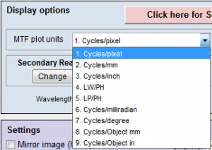
Figure 8. Spatial frequency units are selected in the Settings or More settings windows of SFR and Rescharts modules (SFRplus, eSFR ISO, Star, etc.).

Trull, A. K. et al. Point spread function based image reconstruction in optical projection tomography. Phys. Med. Biol. 62(19), 7784 (2017).

Lee, K. et al. Visualizing plant development and gene expression in three dimensions using optical projection tomography. Plant Cell 18, 2145–2156 (2006).

The high contrast (≥40:1) recommended in the old ISO 12233:2000 standard produced unreliable results (clipping, gamma issues, excessive sharpening with bilateral filters). The new ISO 12233:2014 standard recommends 4:1 contrast. This is our recommendation (with SFRplus or eSFR ISO) for all new work.

Bright fieldmicroscope advantages and disadvantages

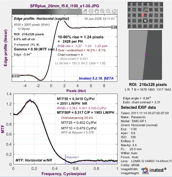
Device or system sharpness is measured as a Spatial Frequency Response (SFR), also called Modulation Transfer Function (MTF). MTF is the contrast at a given spatial frequency (measured in cycles or line pairs per distance) relative to low frequencies. The 50% MTF frequency correlates well with perceived sharpness— much better than the old vanishing resolution measurement, which indicated where the detail wasn’t.

Corresponding summary metrics MTFnn (MTF50, MTF50P, etc.), which have units of frequency, are increased over the initial values.

This new dropdown allows you to choose between Imatest and ISO-compliant calculations.  There are now four options that can be used for SFR Settings to control the Edge SFR Algorithm.

Once the rotation axis is defined we process each plane independently, following an approach that has been proven to work properly in multi-view reconstruction of LSFM data in zebrafish47 and offers the possibility to be accelerated using graphics processing units (GPU), potentially providing the results in real time. Each xz plane is rotated around (xC, zC), by its angle view, and summed to the other views. In total, N different views are summed (N is the number of acquired image stacks around 360°) and the resulting image is divided by N. This mean image is the reconstructed plane. If deconvolution is applied, each xz plane is de-convolved before the sum. For deconvolution we used the theoretical point spread function (PSF) of the microscope. This is generated considering the numerical aperture of the lens, creating the corresponding Ewald sphere33, and calculating the absolute value squared of its 3D Fourier transform. For plane by plane processing, a two dimensional PSF is extracted from its three dimensional counterpart by slicing it in its central section. Deconvolution is then performed using the Wiener or Lucy Richardson filtering in the Python package scikit-image.

(Upper-left)  A narrow image illustrating the tones of the averaged edge. It is aligned with the average edge profile (spatial domain) plot, immediately below.

To overcome this issue, measurements are made in the frequency domain where frequency is measured in cycles or line pairs per distance (millimeters, inches, pixels, image height, or sometimes angle [degrees or milliradians]).

Measurements of zebrafish embryos demonstrate that the whole organism can be acquired in a single experiment. Again, the technique offers the possibility to observe several organs (e.g. notochord, yolk, eye, brain) in single sections (Fig. 5a–c and Supplementary Fig. 4) and within the entire sample anatomy. The use of 4 days post fertilization (dpf) transgenic VEGFR2:GFP zebrafish embryos that express green fluorescent protein under the control of the vascular endothelial promoter VEGFR2/KDR [Tg(kdrl:GFP)]42, confirms that the combination of LSFM and BF reconstruction is a suitable tool to localize a sparse fluorescence signal in the tissue (Fig. 5d–f).

Swoger, J., Verveer, P., Greger, K., Huisken, J. & Stelzer, E. H. Multi-view image fusion improves resolution in three-dimensional microscopy. Opt. Express 15, 8029–8042 (2007).

Hyung-Taeg, C. & Cosgrove, D. J. Regulation of root hair initiation and expansin gene expression in Arabidopsis. Plant Cell 14(12), 3237–3253 (2002).

The MTF calculation is derived from ISO standard 12233. The Imatest calculation contains a number of enhancements, listed below. The original ISO calculation is performed when the ISO standard SFR checkbox in the SFR input dialog box is checked (we recommended leaving it unchecked unless it’s specifically required).

System sharpness is affected by the lens (design and manufacturing quality, position in the image field, aperture, and (for zoom lenses) focal length), sensor (pixel count and anti-aliasing filter), and signal processing (especially sharpening and noise reduction). In the field, sharpness is affected by camera shake (a good tripod can be helpful), focus accuracy, and atmospheric disturbances (thermal effects and aerosols).

FL can be calculated from the simple lens equation*, \(1/FL = 1/s_1 + 1/s_2\), where s1 is the lens-to-chart distance (easy to measure), s2 is the lens-to-sensor distance, and magnification \(M = s_2/s_1\).

2014214 — Made in the USA, the Champ Mobile Inspection Light provides maximum lighting for detailed inspection for paint flaws and body damage.

The sample is rotated by \(\Delta \alpha\) and the previous points are repeated for multiview acquisition. Typically the angle \(\Delta \alpha\) is chosen so to have a full 360° rotation after N + 1 rotation steps.

Imatest‘s primary sharpness measurement uses slanted-edge patterns analyzed by SFRplus, eSFR ISO , SFRreg, or Checkerboard which have automated region detection. SFR, can be used for manually selected SFR regions. Analysis can be performed on targets you can purchase or print with the Imatest Test Charts module. Concise instructions are found in How to test lenses with Imatest.

Past film camera lens tests used line pairs per millimeter (lp/mm), which worked well for comparing lenses because most 35mm film cameras have the same 24 x 36mm picture size. But digital sensor sizes vary widely—from under 5mm diagonal in camera phones to 43mm diagonal for full-frame cameras to an even larger diagonal for medium format. For this reason, line widths per picture height (LW/PH) is recommended for measuring the total detail a camera can reproduce. Note that LW/PH is equal to 2 × lp/mm × (picture height in mm).

Open Access This article is licensed under a Creative Commons Attribution 4.0 International License, which permits use, sharing, adaptation, distribution and reproduction in any medium or format, as long as you give appropriate credit to the original author(s) and the source, provide a link to the Creative Commons license, and indicate if changes were made. The images or other third party material in this article are included in the article’s Creative Commons license, unless indicated otherwise in a credit line to the material. If material is not included in the article’s Creative Commons license and your intended use is not permitted by statutory regulation or exceeds the permitted use, you will need to obtain permission directly from the copyright holder. To view a copy of this license, visit http://creativecommons.org/licenses/by/4.0/.

Arranz, A. et al. In-vivo optical tomography of small scattering specimens: time-lapse 3D imaging of the head eversion process in Drosophila melanogaster. Sci. Rep. 4, 7325 (2014).

Zebrafish AB strains obtained from the Wilson lab (University College London, London, UK) were maintained at 28 °C on a 14 h light/10 h dark cycle. The zebrafish transgenic Tg(kdrl:GFP) was used for fluorescence imaging. Embryos were collected by natural spawning, staged according to Kimmel and colleagues, and raised at 28 °C in fish water (Instant Ocean, 0.1% Methylene Blue) in Petri dishes, according to established techniques. After 24 hpf, to prevent pigmentation 0.003% 1-phenyl-2-thiourea (PTU, Sigma-Aldrich, Saint Louis, MO, USA) was added to the fish water. Embryos were washed, dechorionated and anaesthetized, with 0.016% tricaine (Ethyl 3-aminobenzoate methanesulfonate salt; Sigma-Aldrich, before acquisitions. During imaging, the fish were restrained in FEP (Fluorinated ethylene propylene) tubes37.

Bassi, A., Fieramonti, L., D’Andrea, C., Valentini, G. & Mione, M. In vivo label-free three-dimensional imaging of zebrafish vasculature with optical projection tomography. J. Biomed. Opt. 16(10), 100502 (2011).

Search of the rotation axis. Minimum intensity projection (each pixel shows the minimum value of the stack calculated along the z direction) of the stack acquired at the angle 0° (a). Minimum intensity projection of the stack acquired at the angle 180° (b). The image shown in b, is flipped horizontally and translated to overlap the image in a. The distance Δx/2 indicates the position of the rotation axis from the image center, along the horizontal direction (c). Blurring artifacts arising from incorrectly identified axial position of the rotational axis zC (d–f). The contrast of a series of test reconstructions (g) has a maximum at the position corresponding to the correct rotational axis (zC = 0). Scale bars: 50 µm.

Multimodal acquisition (bright-field/fluorescence) is performed alternating the LED (for trans-illumination) and the laser (for LSFM). After each axial scan required for bright-field acquisition, a second axial scan is repeated for LSFM acquisition. To this end two custom-made mechanical shutters are used to alternate the illuminations.

Candeo, A., Doccula, F. G., Valentini, G., Bassi, A. & Costa, A. Light sheet fluorescence microscopy quantifies calcium oscillations in root hairs of Arabidopsis thaliana. Plant Cell Physiol 58(7), 1161–1172 (2017).

Fieramonti, L. et al. Quantitative measurement of blood velocity in zebrafish with optical vector field tomography. J. Biophotonics 8(1–2), 52–59 (2015).

Offers numerous advantages over the old ISO 12233:2000 test chart: automatic feature detection, lower contrast for improved accuracy, more edges (less wasted space) for a detailed map of MTF over the image surface.

Angular frequencies. Pixel spacing or pitch must be entered. Focal length (FL) in mm is usually included in EXIF data in commercial image files. If it isn’t available it must be entered manually, typically in the EXIF parameters region at the bottom of the settings window. If pixel spacing or focal length is missing, units will default to Cycles/Pixel. Cycles/degree is useful for comparing camera systems to the human eye, which has an MTF50 of roughly 20 Cycles/Degree (depending on the individual’s eyesight and illumination).

Chen, L. et al. Mesoscopic in vivo 3-D tracking of sparse cell populations using angular multiplexed optical projection tomography. Biomed. Opt. Express 6, 1253–1261 (2015).

The optical setup for BF reconstruction is similar to an OPT system1,37,38 except for two main adjustments: (1) a translation stage is required to scan the sample along the optical axis or to scan the detection optics along the sample; (2) the illumination numerical aperture should match that of the detection: \(NA_{ILL} = NA_{DET}\). This second point is recommended to maximize the resolution of the microscope, which according to Abbe is \(\frac{\lambda }{{NA_{ILL} + NA_{DET} }}\), and consequently to obtain reconstructions with higher-contrast.

(Bottom-left) MTF (Frequency domain): The Spatial Frequency Response (MTF), shown to twice the Nyquist frequency. Key summary results include MTF50, the frequency where contrast falls to 50% of its low frequency value, and MTF50P, the frequency where contrast falls to 50% of its peak value, which corresponds well with perceived image sharpness. Units are cycles per pixel (C/P) and Line Widths per Picture Height (LW/PH). Other results include MTF at Nyquist (0.5 cycles/pixel; sampling rate/2), which indicates the probable severity of aliasing and user-selected secondary readouts, and Secondary readouts. The Nyquist frequency is displayed as a vertical blue line. The diffraction-limited MTF response is shown as a pale brown dashed line when the pixel spacing is entered (manually) and the lens focal length is entered (usually from EXIF data, but can be manually entered).

Some lost sharpness can be restored by sharpening, but sharpening has limits. It can’t restore detail where MTF is very low (under about 10%). Oversharpening, illustrated on the right, can also degrade image quality (especially at large magnifications) by causing “halos” to appear near contrast boundaries. Images from many compact digital cameras and phones are oversharpened.

To correctly normalize MTF at low spatial frequencies, a test chart must have some low-frequency energy. This is supplied by large light and dark areas in slanted edges and by features in most patterns used by Imatest, but is not present in lines and grids. For systems where sharpening can be controlled, the recommended primary MTF calculation is the slanted-edge, which is calculated from the Fourier transform of the impulse response (i.e., response to a narrow line), which is the derivative (d/dx or d/dy) of the edge response. Fortunately, you don’t need an understanding of Fourier transforms to understand MTF.

The simplest focal length definition is a description of the distance between the center of a lens and the image sensor when the lens is focused at infinity.

Darkfieldmicroscope

Note: The USAF 1951 chart (long-since abandoned by the Air Force) is poorly suited for computer analysis because it uses space inefficiently and its bar triplets lack a low frequency reference. Furthermore, small changes in chart position (sampling phase) can cause the appearance of its bars to change as they shift from being in phase to out of phase with the pixel array. This adversely affects the vanishing resolution estimate.

Istituto di Fotonica e Nanotecnologie, Consiglio Nazionale delle ricerche, piazza Leonardo da Vinci 32, 20133, Milan, Italy

A Köhler illuminator is used for trans-illumination of the sample. The light source is a LED (Thorlabs M530L2) emitting at 530 nm. The transmitted light is collected by a microscope objective lens (Nikon M = 4×, NADET = 0.13 or Olympus M = 10×, NADET = 0.3) and tube lens to form the image of the sample on a sCMOS camera (Hamamatsu, Flash 4.0). A long pass filter at 500 nm (Thorlabs FEL0500) is placed between the objective lens and the tube lens, suitable for the collection of 530 nm illumination and also for GFP fluorescence detection. The numerical aperture of the Köhler illuminator is matched to that of the detection (NAILL = NADET). The sample is immersed in a cuvette filled with medium from the top, and is translated along the z-axis with a linear stage (Physik Instrument, M-404.1PD) and rotated with a rotation stage (Physik Instrument M-660.55). A manual translator (Thorlabs, ST1XY-S/M) is mounted on the rotation stage to move the sample on the xz plane and position it in the proximity of the rotation axis. This ensures that the specimen is within the field of view at all the acquisition angles. The sample holder and the pre-alignment protocol are described in Bassi et al.22. The experiments are performed with a custom-made light sheet microscope46. For LSFM illumination, a solid-state laser emitting at 473 nm (CNI, MBL-FN-473) is used. The laser beam is expanded to a diameter of 7 mm and split into two portions in order to illuminate the sample from opposite sides: two cylindrical lenses (Thorlabs, LJ1703RM-A, f = 75 mm) are used to create a light sheet made by two counter-propagating beams across the sample. The illumination is perpendicular to the detection path, with the light-sheet formed in the focal plane of the detection objective lens. LSFM and bright-field reconstruction share the same detection system and the acquisition protocol is the same for the two modalities.

EJ Warrant · 2010 · 34 — Two years ago, however, circular polarisation vision was discovered in a mantis shrimp (or stomatopod) — not only does the cuticle of this species reflect.

Mayer, J. et al. OPTiSPIM: integrating optical projection tomography in light sheet microscopy extends specimen characterization to non-fluorescent contrasts. Opt. Lett. 39(4), 1053–1056 (2014).

MTF curves and Image appearance contains several examples illustrating the correlation between MTF curves and perceived sharpness.

*For SFRplus when bar-to-bar spacing is entered, eSFR ISO when the registration mark vertical spacing is entered, or Checkerboard when the square length is entered, Cycles per object distance is calculated directly without using pixel spacing or entering magnification, which is calculated from the geometry. Before Imatest 2021.2 you had to enter a number in the Pixel spacing field, but this number is not used for the actual calculation. We apologize for the confusion.

New in Version 22.1 – an Imatest/ISO Standard SFR dropdown menu is located on the lower left of slanted-edge More Settings window. (This option was formerly a checkbox for “ISO compatible” calculations),

In principle, MTF measurements should be the same when no nonuniform or nonlinear image processing (bilateral filtering) is applied, for example when the image is demosaiced with dcraw or LibRaw with no sharpening and noise reduction. But this does not exactly happen because demosaicing, which is present in all cameras that use Color Filter Arrays (CFAs) involves some nonlinear processing. The sensitivity of different patterns to image processing is summarized in the image below.

Better indicators of image sharpness are spatial frequencies where MTF is 50% of its low frequency value (MTF50) or 50% of its peak value (MTF50P). MTF50 and MTF50P are recommended for comparing the sharpness of different cameras and lenses because

Remarkably, transmission OPT, which provides bright-field contrast, is used to correct absorption artifacts in Light Sheet Fluorescence Microscopy (LSFM)20,21 and for multimodal reconstruction of the whole specimen’s anatomy22.

Setting #2 (ISO 12233 2017 & earlier) is not recommended because the Imatest and newer ISO calculations are more accurate— definitely superior in the presence of noise and optical distortion. More information on calculations can be found below:

Bright fieldmicroscope diagram

Comparison of the effects of image processing (bilateral filtering) on MTF measurements: Slanted-edges and wedges tend to be sharpened the most. The random 1/f pattern has the least sharpening and the most noise reduction.

Sharpe, J. et al. Optical projection tomography as a tool for 3D microscopy and gene expression studies. Science 296, 541–545 (2002).

Walls, J. R., Sled, J. G., Sharpe, J. & Henkelman, R. M. Correction of artefacts in optical projection tomography. Phys. Med. Biol. 50(19), 4645–4665 (2005).

The project has received funding from the European Union’s Horizon 2020 research and innovation programme under grant agreement no. 871124.

As described and characterized by Trull et al.24, the diffraction of light in OPT causes space-variant tangential blurring that increases with the distance from the rotation axis. We clearly observe these artifacts when imaging structures that are just hundreds of microns away from the rotation axis. This effect is shown in the completely distorted reconstruction (Fig. 2a, blue arrow) of a root hair of Arabidopsis thaliana, which is c.a 200 µm away from the rotation axis (located at the center of the OPT reconstructed section in Fig. 2a). In Fig. 2, the sample was embedded in a tube (see Material and Methods) that is visible in the OPT reconstruction due to the presence of a small amount of scattering which causes light attenuation. The size of the tube can be used as a benchmark to assess the presence of space-variant blurring. We observe that the higher the distance from the center of rotation, the more blurred the border of the tube is in the OPT reconstruction. When applying the multi-view approach, the sample is reconstructed correctly in the entire field of view, avoiding the diffraction artifacts (Fig. 2b). However, as expected, by simply overlapping (sum) the views acquired at different angles, the image is overall blurred. In order to increase the quality of the reconstruction we used a deconvolution approach based on the Wiener or Lucy Richardson methods (see Material and Methods). In this way, the contrast and resolution are significantly improved leading to the observation of the Arabidopsis section at single cell detail (Fig. 2c). This improvement comes at the expense of higher noise, and in order to fully exploit the capabilities of the method a systematic study on deconvolution and regularization should still be carried out. It is worth noting that in case of highly diffusive samples the technique would be able to reconstruct only the outermost part of the specimen with artifacts given by the diffusion of light. Therefore, the method should be applied to translucent samples (as it is the case for zebrafish embryos and Arabidopsis roots), chemically cleared samples, or it should be combined with more advanced methods to reduce the effect of diffusion34,35,39.

The idea behind OPT is to acquire images (or projections) of the sample from different orientations. Similarly to X-ray CT the sample is then reconstructed using a back-projection algorithm23. However, this algorithm assumes that the light beam propagates straight through the sample: in X-ray CT the straight propagation is given by the high frequency of the radiation, whereas in OPT we can consider a straight propagation of light only within the depth of field of the system. Since the depth of field scales with the inverse of the second power of the Numerical Aperture (NA), the assumption is valid only at low NA (c.a < 0.1) which typically corresponds to a low magnification (1×, 2×). At higher NAs, artifacts due to the diffraction of light are present24. One way to attenuate these artifacts consists in limiting the NA of the microscope (e.g. by inserting a diaphragm at the back focal plane of the detection objective), but this also limits the resolution. Another way to mitigate this effect is to incorporate a spatially variant deconvolution in the reconstruction algorithm24,25. To drastically remove the diffraction artifact, some methods based on the extension of the depth of field have been proposed21,26,27,28. For each projection, the sample is scanned at different positions (up to 100) along the optical axis, and the acquired stack of images is merged into a single entirely focused projection29. Yet, this come at the expenses of the number of acquired images, since the process must be repeated for each projection (up to 1,000 angles within 360° rotation).

Dipartimento di Biotecnologie Mediche e Medicina Traslazionale, Università degli Studi di Milano, via Fratelli Cervi 93, 20090, Segrate, Italy

Edge Contrast should be limited to 10:1 at the most, and a 4:1 edge contrast is generally recommended. The reason is that high contrast edges (>10:1, such as found in the old ISO 12233:2000 chart) can cause saturation or clipping, resulting in edges with sharp corners that exaggerate MTF measurements. For more details, see Using Rescharts slanted-edge modules, Part 2: Warnings – clipping.

Bryson-Richardson, R. & Currie, P. Optical projection tomography for spatio-temporal analysis in the zebrafish. Methods Cell Biol. 76, 37–50 (2004).

After seedling germination and fluorescence inspection, the germinated fluorescent seeds were moved from the plate to the top of FEP tubes filled with gel (prepared accordingly to Candeo et al.,43 and Romano Armada et al.45, using sterilized pliers and without clamping them, so the plantlets could grow inside the filled tubes. The tubes were transferred to a tip box that was finally filled with MS/2 liquid medium without sucrose and sealed to avoid contamination. The mounting procedure and the special illumination and detection configuration of OPT-LSFM allowed the seedlings to be held from the top of the chamber in a vertical position, with the roots growing directly in the jellified medium inside the transparent tubes. To mount the tubes with the plant in the imaging chamber, we used the custom holder reported in Candeo et al.43. When plants were ready to be imaged, we plugged the pipette tip with the tube into the holder, and quickly moved it to the imaging chamber, fixing it on a rotation and translation stage for the sample positioning.

202463 — For example, a M12 4-pin A-coded connector is designed for sensor signals, while a M12 4-pin D-coded connector is used for industrial Ethernet.

Candeo, A. et al. Virtual unfolding of light sheet fluorescence microscopy dataset for quantitative analysis of the mouse intestine. J. Biomed. Opt. 21(5), 056001 (2016).

Arabidopsis thaliana seedling preparation was carried out accordingly to Candeo et al.43,44. and Romano Armada et al.45. Briefly, seeds of Arabidopsis thaliana Col-0 transformed with pEXP7:YC3.6 were surface sterilized by vapour-phase sterilization and plated on MS/2 medium supplemented with 0.1% (w/v) sucrose, 0.05% (w/v) MES, pH 5.8 adjusted with KOH and solidified with 0.8% (w/v) plant agar (Duchefa, The Netherlands). After stratification at 4 °C in the dark for 2–3 days, seeds were transferred to the growth chamber with 16/8 h cycles of light (70 µmol m−2 s−1) at 24 °C.

The ISO 12233 standard recommends an angle of either 5 or 5.71 degrees (arctan(0.1)). This angle is not sacred— MTF is not strongly dependent on edge angle. Angles from 3 to 7 degrees work fine. For nonzero edge angles θ relative to the closest V or H orientation, a cosine correction is applied, as illustrated on the right. The correction is significant when θ is greater than about 8 degrees (cos(8º) = 0.99). The initial MTF and corresponding frequency f are calculated from a Vertical or Horizontal line (shown in blue), based on the region selection. The true MTF is defined normal to the edge— along the red line. Since the length of the actual transition along the red line (normal to the edge) is shorter than the measured transition along the blue (V or H) line, and since the frequency f used to measure MTF is inversely proportional to the actual transition length,

The system required for BF multi-view reconstruction consists in a trans-illumination microscope in which the sample can be rotated over 360° (around the y axis in Fig. 1a) and translated along the optical axis (axis z in Fig. 1a). Like any wide-field microscope, the system presents a limited optical sectioning capability which is a consequence of the so called “missing cone” in the Optical Transfer Function (OTF)33 (Fig. 1b). For this reason, if we acquire a stack of images of the sample at different axial positions, the three-dimensional reconstruction that we obtain will have a limited axial resolution. We observe for example that the transverse section of a sample (an Arabidopsis thaliana root), presents such a poor axial resolution (Fig. 1c, left hand side) that different structures are indistinguishable, hindering any 3D analysis of the sample.

Measures MTF and other image quality parameters from Imatest SFRplus chart (recommended) or created using Imatest Test Charts (a wide-body printer, advanced printing skills, and knowledge of color management required).

Measures MTF and other image quality parameters using an enhanced version of the ISO 12233:2014 and 2017 Edge SFR (E-SFR) test chart

To calculate the exit pupil, divide the size of the objective lens by the magnification of the riflescope. For example, the exit pupil of a 3-15x56 is 18.6 at ...

Secondly, to determine the location zC of the rotational axis along the z axis, we adopted an approach typically used in OPT38. We select a single transverse section of the sample (in a certain y location), reconstruct the section assuming different zC values and calculate the contrast of each reconstruction (Fig. 3d–g), as described in Material and Methods. The reconstructed image that has the highest contrast is the closest to the ideal reconstruction, as it is the least blurred. The corresponding zC position is considered to be that of the rotation axis.

Linearly polarized light is a special case of elliptically polarized light. If the light is linearly polarized, then the two components oscillate in phase, for ...

Fauver, M. et al. Three-dimensional imaging of single isolated cell nuclei using optical projection tomography. Opt. Express 13, 4210–4223 (2005).

Traditional resolution measurements involve observing an image of bar patterns, most frequently the USAF 1951 chart (Figure 7) and estimating the highest spatial frequency (lp/mm) where bar patterns are visibly distinct. This observation (also called vanishing resolution) corresponds to an MTF of roughly 10-20%. Because the vanishing resolution is the spatial frequency where image information disappears— where it isn’t visible, it is strongly dependent on observer bias and is a poor indicator of image sharpness. (It’s Where the Woozle Wasn’t in Winnie the Pooh.)

On the other hand, the system required for BF reconstruction is also commonly present in multi-view LSFM microscopes, which allow translation and rotation of the specimen. Therefore, we performed our analysis on a LSFM microscope equipped with a Köhler illuminator for trans-illumination. In particular we used a 4× magnification (NA = 0.13) in the detection path: at this magnification and NA, the artifacts given by the diffraction are already present and significantly compromise the standard OPT results (Fig. 2a).

van der Horst, J. & Kalkman, J. Image resolution and deconvolution in optical tomography. Opt. Express 24(21), 24460–24472 (2016).

Bassi, A., Fieramonti, L., D’Andrea, C., Mione, M. & Valentini, G. In vivo label-free three-dimensional imaging of zebrafish vasculature with optical projection tomography. J. Biomed. Opt. 16, 100502 (2011).

Alanentalo, T. et al. Tomographic molecular imaging and 3D quantification within adult mouse organs. Nat. Methods 4, 31–33 (2007).

MTF results for pure vertical or horizontal edges are highly dependent on sampling phase (the relationship between the edge and the pixel locations), and hence can vary from one run to the next depending on the precise (sub-pixel) edge position. The edge is slanted so MTF is calculated from the average of many sampling phases, which makes results much more stable and robust (Figure 9).

Andrews, N. et al. Visualising apoptosis in live zebrafish using fluorescence lifetime imaging with optical projection tomography to map FRET biosensor activity in space and time. J. Biophotonics 9(4), 414–424 (2016).

With this technique, sharpness can be determined by the distance of a pixel level between 10% to 90% of its final value (also called 10-90% rise distance; see Figure 3).

Bright fieldmicroscope principle

The reconstruction consists in a multi-view fusion of the data acquired at different angles. Data processing was performed in Python; a sample code is available on GitHub (https://github.com/andreabassi78/BrightfieldMultiviewReconstruction).

Boot, M. J. et al. In vitro whole-organ imaging: 4D quantification of growing mouse limb buds. Nat. Methods 7, 609–612 (2008).

Visualizing Sharpness | Rise Distance and Frequency Domain | Modulation Transfer Function | Spatial Frequency Units  Summary metrics | MTF measurement Matrix| Slanted-Edge measurement | Edge angles | Slanted-Edge modules  Edge contrast and clipping | Slanted-Edge algorithm | Differences with ISO | Noise reduction  Related sharpness techniques | Key takeaways | Additional resources

Cycles per distance on the object being photographed (what some people think of as the “subject”). Pixel spacing and magnification must be entered with an important exception*. Should be used when the system specification references the object being photographed (for example, if features of a certain width need to be detected). Recommended for object-centric applications in Comparing sharpness in different cameras.

All methods were carried out in accordance with relevant guidelines and regulations. Zebrafish (Danio rerio) were maintained at the zebrafish facility, University of Milan, Via Celoria 26—20133 Milan, Italy (Aut. Prot, n. 295/2012-A—20/12/2012 for the breeding, growth and use of zebrafish, released by the Azienda di Tutela della Salute, ATS Città metropolitana di Milano). All experimental procedures were performed according to the international (EU Directive 2010/63/EU) and national guidelines (Italian decree No 26 of the 4th of March 2014). Embryos were staged and used until 5 days post fertilization, a time windows in which zebrafish is not considered an animal model according to national guidelines (Italian decree No 26 of the 4th of March 2014). All procedures to minimize stress and pain of the embryos were applied. Embryos were anaesthetized with 0.016% tricaine (Ethyl 3-aminobenzoate methanesulfonate salt, Sigma-Aldrich) before proceeding with experimental protocols.

Costa, A., Candeo, A., Fieramonti, L., Valentini, G. & Bassi, A. Calcium dynamics in root cells of Arabidopsis thaliana visualized with selective plane illumination microscopy. PLoS ONE 8, e75646 (2013).

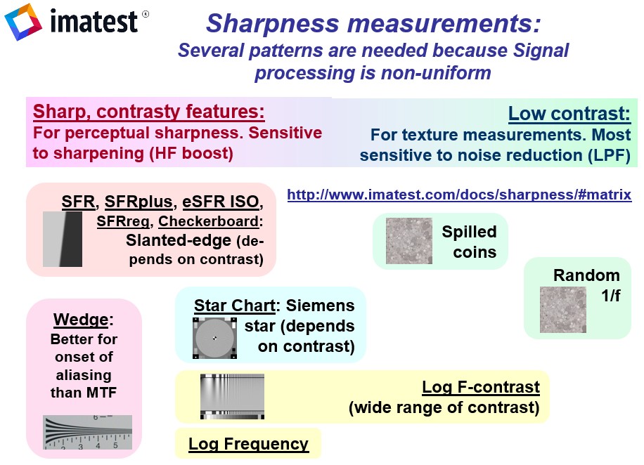
Although MTF can be estimated directly from images of sine patterns (using Rescharts,Log Frequency, Log F-Contrast, and Star Chart), the ISO 12233 slanted-edge technique provides more accurate and repeatable results and uses space more efficiently.  Slanted-edge images can be analyzed by one of the modules listed in the MTF Measurement Matrix, below.

Spatial frequency is measured in cycles (or line pairs) per distance instead of time. As with temporal (e.g., audio) frequency response, the more extended the response, the more detail can be conveyed.

The key output of slanted edge analysis is the Edge/MTF plot, which can be viewed by clicking the button below. Many additional results are available, including summary and 3D plots, showing Lateral Chromatic Aberration and other results as well as MTF.

Cross, L. M., Cook, M. A., Lin, S., Chen, J. N. & Rubinstein, A. L. Rapid analysis of angiogenesis drugs in a live fluorescent zebrafish assay. Arterioscler. Thromb. Vasc. Biol. 23, 911–912 (2003).

Optical Projection Tomography (OPT) is a powerful three-dimensional imaging technique used for the observation of millimeter-scaled biological samples, compatible with bright-field and fluorescence contrast. OPT is affected by spatially variant artifacts caused by the fact that light diffraction is not taken into account by the straight-light propagation models used for reconstruction. These artifacts hinder high-resolution imaging with OPT. In this work we show that, by using a multiview imaging approach, a 3D reconstruction of the bright-field contrast can be obtained without the diffraction artifacts typical of OPT, drastically reducing the amount of acquired data, compared to previously reported approaches. The method, purely based on bright-field contrast of the unstained sample, provides a comprehensive picture of the sample anatomy, as demonstrated in vivo on Arabidopsis thaliana and zebrafish embryos. Furthermore, this bright-field reconstruction can be implemented on practically any multi-view light-sheet fluorescence microscope without complex hardware modifications or calibrations, complementing the fluorescence information with tissue anatomy.

To accurately reconstruct the data, the position of the rotation axis must be determined at pixel resolution. We propose a straightforward method based on two processing steps to locate the rotation axis, both in x and z, assuming that the latter is parallel to the y axis (as in Fig. 1a).

Using BF reconstruction, we managed to acquire a large volume of the biological sample in a single measurement. We tested the method in vivo with Arabidopsis thaliana and zebrafish (Danio rerio) samples. In the root of Arabidopsis seedlings, the reconstruction can be extended to a large portion of the root including the root hairs, which are long tubular-shaped outgrowths from root epidermal cells (Fig. 4 and Supplementary Fig. 3). One key feature of the technique is to provide isotropic resolution over the entire reconstructed volume. In addition, the method is label-free, since the BF reconstruction is based on trans-illumination. In living samples, the contrast is given by the attenuation of light, primarily due to scattering and absorption. Therefore, while on the one hand the staining is not required for imaging, on the other hand, since low-power light sources are used for trans-illumination, the measurements induce minimum photo-toxicity to the biological sample. These features make the technique an ideal tool for assessing the anatomy of the sample in-vivo.

Download bx logo stock vectors. Affordable and search from millions of royalty free images, photos and vectors.

Note: Imatest uses SFR and MTF interchangeably. SFR is more commonly associated with complete system response, where MTF is commonly associated with the individual effects of a particular component. In other words, system SFR is equivalent to the product of the MTF of each component in the imaging system.

Bright fieldmicroscope

High spatial frequencies (on the right) correspond to fine image detail. The response of photographic components (film, lenses, scanners, etc.) tends to “roll off” at high spatial frequencies. These components can be thought of as low-pass filters that pass low frequencies and attenuate high frequencies.

Comparing sharpness in different cameras recommends spatial frequency units based on one of two broad types of application:

Most readers will be familiar with temporal frequency. For example, the frequency of a sound—measured in Cycles/Second or Hertz—is closely related to its perceived pitch. The frequencies of radio transmissions (measured in kilohertz, megahertz, and gigahertz) are also familiar.

In this case, the theoretical number of acquired views is \(N = \frac{2\pi n}{{NA}} \approx 48\) and the theoretical axial step is \(\Delta z = \frac{\lambda n}{{NA^{2} }} \approx 30 \;\upmu {\text{m}}\) (here λ = 530 nm). For a sample of thickness L = 300 µm the number of steps results in M ≈ 10. The results of the reconstruction performed for different values of N and M (Supplementary Fig. 1) confirm that the theoretical values are a good estimate: above N = 45 and M = 10 the increase in image contrast is negligible. The number of required views is therefore an order of magnitude smaller than the number of projections in standard OPT. Yet, the total amount of data remains practically constant because for each view a stack of images is required, but overall the acquisition time is comparable to that of standard OPT (1–5 min per sample).

Imatest Slanted-Edge Modules include SFR, SFRplus, eSFR ISO, Checkerboard, and SFRreg (see Table 2 and Sharpness Modules for details).

The relative contrast at a given spatial frequency (output contrast/input contrast) is called Modulation Transfer Function (MTF), which is similar to the Spatial Frequency Response (SFR), and is a key to measuring sharpness. In Figure 6, MTF is illustrated with sine and bar patterns, an amplitude plot, and a contrast plot—each of which has spatial frequencies that increase continuously from left to right.

Figure 8. Spatial frequency units are selected in the Settings or More settings windows of SFR and Rescharts modules (SFRplus, eSFR ISO, Star, etc.).

(Middle-left) Average Edge (Spatial domain): The average edge profile shown here linearized (the default). A key result is the edge rise distance (10-90%), shown in pixels and in the number of rise distances per Picture Height. Other parameters include overshoot and undershoot (if applicable). This plot can optionally display the line spread function (LSF: the derivative of the edge).

Thank you for visiting nature.com. You are using a browser version with limited support for CSS. To obtain the best experience, we recommend you use a more up to date browser (or turn off compatibility mode in Internet Explorer). In the meantime, to ensure continued support, we are displaying the site without styles and JavaScript.

Both Dead Leaves (Spilled Coins) and Random charts are analyzed with the Random (Dead Leaves) module. Strong bilateral filtering can cause misleading results.

The primary disadvantage of large edge angles is that the available region area may be reduced, especially for SFRreg patterns.

Fieramonti, L. et al. Time-gated optical projection tomography allows visualization of adult zebrafish internal structures. PLoS ONE 7(11), e50744 (2012).

Figure 1. Bar pattern: Original (upper half of figure) with lens degradation (lower half of figure) Figure 2. Sharpness example on image edges from MTF Curves and Image Appearance

Then, stacks acquired at the different angles are resliced into planes (xz) which are orthogonal to the rotation axis. The z location of the center of rotation is found by maximizing the contrast of the reconstruction at different possible zC. The contrast is calculated as the energy (sum) of all the frequency components obtained by numerically Fourier transforming (fft2 function in the Python module numpy) the reconstruction, excluding the DC component.

2023630 — automatica 2023. Visit us in Hall B6 Booth 509 and discover how our groundbreaking technology boosts efficiency by 30%. Date: June 27th ...

Imatest has many patterns for measuring MTF— slanted-edge, Log frequency, Log f-contrast, Siemens Star, Dead Leaves (Spilled Coins), Random 1/f, and Hyperbolic wedge— each of which tends to give different results in consumer cameras, most of which have nonuniform image processing— commonly bilateral filtering— that depends on local scene content. Sharpening (high frequency boost) tends to be maximum near contrasty features (larger near higher contrast edges), while noise reduction (high frequency cut, which can obscure fine texture) tends to be maximum in their absence. For this reason MTF measurements can be very different with different test charts.

PH = Picture Height in pixels. FL(mm) = Lens focal length in mm.  Pixel pitch = distance per pixel = 1/(pixels per distance).   Note: Different units scale differently with image sensor and pixel size.

In summary we have shown that three-dimensional reconstructions of unstained samples can be achieved in multi-view microscopes, with isotropic resolution, typical of OPT, but without the diffraction artifacts that affect OPT reconstruction. The bright-field multi-view reconstruction provides a comprehensive picture of zebrafish and Arabidopsis thaliana anatomy, including organs that are usually not labelled and therefore not observable. The bright-field contrast nicely complements the fluorescence contrast observable with LSFM, allowing correlative fluorescent protein expression and anatomical visualization.

Sharpness is arguably the most important single image quality factor: it determines the amount of detail an image can convey. The image on the upper right illustrates the effects of reduced sharpness (from running Image Processing with one of the Gaussian filters set to 0.7 sigma).

This approach assumes that the rotation axis is perfectly perpendicular to the optical axis of the detection objective. If this is not the case, we suggest to repeat the procedure at two or more y locations and then linearly interpolate the values of xC and zC for all the considered y values.

Bright fieldmicroscope application

Note: Origins of Imatest slanted-edge SFR calculations were adapted from a Matlab program, sfrmat, which was written by Peter Burns to implement the ISO 12233:2000 standard. Imatest’s SFR calculation incorporates numerous improvements, including improved edge detection, better handling of lens distortion, and better noise immunity. The original Matlab code is available here. In comparing sfrmat results with Imatest, tonal response is assumed to be linear; i.e., gamma = 1 if no OECF (tonal response curve) file is entered into sfrmat. Since the default value of gamma in Imatest is 0.5, which is typical of digital cameras in standard color spaces such as sRGB, you must set gamma to 1 to obtain good agreement with sfrmat.

Sagittal slice of a transgenic Tg(kdrl:GFP) zebrafish (4 dpf) visualized with bright-field multi-view reconstruction (a). Details of the sample showing a portion of the head (b) and of the zebrafish notochord (c). Minimum intensity projection of the bright-field reconstruction (grey) overlapped with the maximum intensity projection of the LSFM data (green). The bright-field reconstruction shows the whole zebrafish anatomy while LSFM shows the labelled vasculature (d). Transverse section of the sample in the head (e) and tail (f), showing the bright-field reconstruction (grey) and LSFM (green). Scale bars: 100 µm.

Cheddad, A., Svensson, C., Sharpe, J., Georgsson, F. & Ahlgren, U. Image processing assisted algorithms for optical projection tomography. IEEE Trans. Med. Imaging 31(1), 1–15 (2012).

Several methods are used for measuring sharpness that include the 10-90% rise distance technique, modulation transfer function (MTF), special and frequency domains, and slanted-edge algorithm.

Experimental setup for multi-view bright-field reconstruction: an LED (530 nm) illuminates the sample, the transmitted light is collected by a detection optical system and a camera. The sample is mounted on a translation and a rotation stage to be scanned and rotated around 360°. A stack of images is acquired in each angular position while scanning the sample (a). Scheme of the Optical Transfer Function of the microscope (b, upper panel). Acquiring multiple views is equivalent to rotating the OTF and sampling different spatial frequencies (b, lower panel). Reconstruction of the transverse section of a sample (Arabidopsis thaliana) using a single view (0°), 10 views (covering 60° in total) and 60 views (covering 360°), each with a spacing of 6°. The illumination and detection numerical aperture is NA = 0.13 (c). Scale bar: 50 µm.

G.C. and A.B designed the experiments. G.C., A.B., C.D., A.Ca, A.F., V.M. and G.V. acquired and analyzed the data, A.Co. and A.P. prepared the samples and developed the imaging protocol. A.B. wrote the manuscript.

Bright fieldmicroscope image

*Unless s1 >> s2, (by 100× or more), lens geometry (s1, s2, and FL) is not reliable for calculating M because lenses can deviate significantly from the simple lens equation.

First, two stacks of images are acquired at opposite angles (e.g. 0° and 180°) and the two corresponding projections are created (mean intensity projection or minimum intensity projection, as shown in Fig. 3a, b). One of the two projections is flipped along the x axis and translated to overlap to the other using an image registration algorithm: in order to overlap the two images, the second projection is translated by a distance Δx (Fig. 3c). The location xC of the rotation axis is then calculated as the sum of semi-width of the image and the distance Δx/2.

Reconstruction of a transverse section of an Arabidopsis thaliana root using Optical Projection Tomography (a), bright-field multi-view reconstruction (b) and bright-field multi-view deconvolution (c). For (c, d), 45 views around 360°, with 8° spacing were used. The presence of spatially variant artifacts in OPT is shown with the blue arrow. The red arrows indicate the thickness of the reconstructed plastic tube far from the rotation center of the OPT reconstruction. Scale bar: 100 µm.

Mayer, J., Robert-Moreno, A., Sharpe, J. & Swoger, J. Attenuation artifacts in light sheet fluorescence microscopy corrected by OPTiSPIM. Light Sci. Appl. 7, 70 (2018).

Several summary metrics are derived from MTF curves to characterize overall performance. These metrics are used in a number of displays, including secondary readouts in the SFR/SFRplus/eSFR ISO Edge/MTF plot (see Imatest Slanted-Edge Results) and in the SFRplus 3D maps.

An Edge/MTF plot from Imatest SFR (for an SFRplus chart image) is shown on the right. SFRplus, eSFR ISO, SFRreg, and Checkerboard produce similar results and much more.

At each angle, in order to cover the specimen of thickness \(L\), we acquired M images while translating the sample with a step Δz. Since the maximum axial cutoff frequency 33 of the microscope is \(\Delta k_{z} = \frac{{NA^{2} }}{2\lambda n}\), following the Nyquist’s criterion we scanned the sample with an axial step \(\Delta z = \frac{1}{{2 \Delta k_{z} }} = \frac{\lambda n}{{NA^{2} }}\). The number of acquisitions along z is given by \(M = \frac{L}{\Delta z} = \frac{{L \cdot NA^{2} }}{\lambda n}\). We observe that the total number of acquired images \(N_{TOT} = N \cdot M = \frac{2\pi \cdot L \cdot NA }{{ \lambda }}\) scales linearly with the numerical aperture, indicating that the approach is particularly suitable for numerical apertures and magnifications which are between those normally used in OPT and those used in high-resolution optical microscopy.

Bright fieldmicroscope parts

Here we show that the Bright-Field (BF) contrast can be efficiently reconstructed in 3D by adopting a multi-view image processing method: we propose to fuse three-dimensional image data sets of the sample acquired at multiple angles into a single reconstruction. Each data set consists of a stack of bright-field images acquired by scanning the sample along the optical axis. The method requires the acquisition of a reduced number of angles and eliminates the diffraction artifacts, still providing isotropic resolution and 3D reconstruction of unlabeled samples. The reconstruction is not based on a back-projection algorithm, it uses a multiview fusion approach, that is frequently used in fluorescence imaging30. Here we describe how to apply this approach to reconstruct the BF contrast and we identify the optimal parameters for reconstruction as a function of the spatial and angular sampling. We present in-vivo data of Arabidopsis thaliana and zebrafish (Danio rerio) in order to demonstrate that the approach allows one to observe the whole anatomy of unstained organisms. Finally, we show that, with small modification of the hardware, BF reconstruction can be readily implemented in any multi-view Light Sheet Fluorescence Microscope (LSFM)31,32, obtaining multimodal (bright-field and fluorescence) acquisitions with the same instrument.

Note:  In imaging systems, one cycle (C) is equivalent to one line pair (LP). The two nomenclatures are used interchangeably.

BF reconstruction can be easily implemented in a multi-view light sheet microscope, complementing the high-resolution fluorescence reconstruction obtained with LSFM. In particular, we acquired images from transgenic Arabidopsis seedlings expressing the Cameleon YC3.640 under the control of AtEXP7 promoter (pEXP7:YC3.6) which directs root hair-specific expression (trichoblast cells) of the fluorescent sensor41. This acquisition shows that by combining LSFM with BF reconstruction the fluorescence can be precisely localized in the context of a single tissue sections (Fig. 4c, d) or in the entire volume (Fig. 4e). It is worth noting that the BF reconstruction is performed with a LED illumination at λ = 530 nm, close to the emission wavelength of GFP, avoiding any chromatic aberration (Fig. 4f).

Spatial frequency units can be selected from the Settings or More settings windows of SFR and Rescharts modules (SFRplus, eSFR ISO, Star, etc. Figure 8) and is the measurement intended to determine how much detail a camera can reproduce or how well the pixels are utilized.

Walls, J. R., Coultas, L., Rossant, J. & Henkelman, R. M. Three-dimensional analysis of vascular development in the mouse embryo. PLoS ONE 3, e2853 (2008).

Image Quality Factors for Cameras and Displays Sharpness Noise Dynamic range Color accuracy Distortion Uniformity Blemishes ISO Sensitivity Chromatic Aberration Stray Light (Flare) Moiré Artifacts Compression Losses Dmax (Maximum Density) Color gamut  Texture Detail Summary table — corresponding test charts and modules

Miao, Q. et al. Resolution improvement in optical projection tomography by the focal scanning method. Opt. Lett. 35, 3363–3365 (2010).

Share your videos with friends, family, and the world.

Another useful spatial frequency unit is cycles per pixel (C/P), which gives an indication of how well individual pixels are utilized. The choice of units is also influenced by whether performance at the image (sensor) or on the object has primary importance: see Comparing sharpness in different cameras. There is no need to use actual distances (millimeters or inches) with digital cameras, although such measurements are available (Table 1).

Armada, N. R. et al. In vivo light sheet fluorescence microscopy of calcium oscillations in Arabidopsis thaliana. Methods Mol. Biol. Calcium Signal. 10, 87–101 (2019).

The sample is translated along the optical axis and images are continuously acquired by the camera. The velocity of the linear stage is synchronized with the acquisition so that every captured image corresponds to a linear step of Δz.

In the frequency domain, a complex signal (audio or image) can be created by combining signals consisting of pure tones (sine waves), which are characterized by a period or frequency (Figure 4). The response of a complete system is the product of the responses of each component.

Three-dimensional optical imaging techniques are essential tools for observing the structure and understanding the function of biological samples. Among them Optical Projection Tomography (OPT), is well suited to study specimens ranging in size from hundreds of microns to a centimeter1. OPT is often considered the optical analogous of X-ray Computed Tomography (CT), performing tomographic optical imaging of three dimensional samples with transmitted and fluorescent light. OPT can be used in a number of different applications with specimens that include embryos2,3, mouse organs4,5,6 and plants7. At the same time novel OPT configurations have been presented to achieve fast acquisition8,9,10, to reconstruct the fluorescence lifetime and Förster resonance energy transfer contrast11,12, to obtain the contrast from blood flow13,14,15,16. In parallel, advanced recontruction algorithms have constantly been developed17,18,19.

Several alternative patterns, which cause cameras to apply differing amounts of sharpening and noise reduction, can be used for measuring MTF. All require more real estate than the slanted-edge. They include

202389 — We are excited to significantly enhance our laser optics manufacturing capabilities and capacity with the new Florida facility, says Marisa ...

Where possible, edge angles should be greater than ±2 degrees from the closest Vertical (V), Horizontal (H), or 45 degree orientation. The reason is that results from vertical, horizontal, and 45° edges are very sensitive to the relationship between the edge and the pixels (i.e., they are phase-sensitive). Tilting the edges by more than 2 or 3 degrees avoids this issue.

Bassi, A., Schmid, B. & Huisken, J. Optical tomography complements light sheet microscopy for in toto imaging of zebrafish development. Development 142, 1016–1020 (2015).

The technique performs well also at higher NA. An example of reconstruction at NA = 0.3 with 10× magnification is shown in Supplementary Fig. 2. Here the diffraction artifacts in standard OPT are much stronger and a strategy for extending the depth of field22,27,28 would be in any case required. However, the focus of the present paper is to image an entire sample in a single measurement, which is demonstrated at lower magnification.

Three-dimensional imaging of a transgenic pEXP7:YC3.6 Arabidopsis thaliana seedling. Transverse (a) and lateral (b) sections of root tip (mature zone) acquired with bright-field multi-view reconstruction. Transverse (c) and lateral (d) sections acquired with bright-field reconstruction (grey) and LSFM (green). Maximum intensity projection of the LSFM stack, combined with the minimum intensity projection of the bright-field reconstruction (e). Detail of panel e, showing the outgrowing part of the root-hair epidermal cells (f). Three-dimensional rendering of the reconstructed bright-field volume, combined with LSFM. Scale bar: 100 µm.

The x location of the center of the rotation axis is found by registering two opposite views projections. The registration is performed using the Python module scikit-image (register_translation) to determine the distance Δx (Fig. 3c).

McGinty, J. et al. In vivo fluorescence lifetime optical projection tomography. Biomed. Opt. Express 2(5), 1340–1350 (2011).

Shipping Policy | Privacy Policy | Return Policy | Imatest Terms and Conditions

The perceived sharpness of a print or display is measured by Subjective Quality Factor (SQF) or Acutance, which are derived from MTF, the Contrast Sensitivity Function of the human eye, and viewing conditions.

Calisesi, G., Candeo, A., Farina, A. et al. Three-dimensional bright-field microscopy with isotropic resolution based on multi-view acquisition and image fusion reconstruction. Sci Rep 10, 12771 (2020). https://doi.org/10.1038/s41598-020-69730-4

In Figure 1, sharpness is illustrated with a bar pattern of increasing spatial frequency. The top portion of the figure is sharp and its boundaries are crisp; the lower portion is blurred and illustrates how the bar pattern is degraded after passing through a simulated lens.

Kumar, V., Chyou, S., Stein, J. V. & Lu, T. T. Optical projection tomography reveals dynamics of HEV growth after immunization with protein plus CFA and features shared with HEVs in acute autoinflammatory lymphadenopathy. Front. Immunol. 3, 282 (2012).

Chen, L. et al. Remote focal scanning optical projection tomography with an electrically tunable lens. Biomed. Opt. Express 5(10), 3367–3375 (2014).

Note: Imatest Master can calculate MTF for edges of virtually any angle, though exact vertical, horizontal, and 45° should be avoided because of sampling phase sensitivity.

Rise distance is not widely used because there is no convenient way of calculating the rise distance of an imaging system from the rise distances of its individual components (i.e., lens, digital sensor, and software sharpening).

In order to obtain optical sectioning, we acquired multiple views of the specimen separated by an angle Δα and at each angle we collected a stack of images with sampling steps Δz. The different stacks were fused together to create a single reconstruction of the sample. We estimated the required number N of views by looking at the system OTF (Fig. 1b). Considering that, in paraxial approximation, the angle θ subtended by the OTF is approximately the system numerical aperture \(NA = n sin\theta \approx n\theta\) (where n is the index of refraction), we chose to acquire the views at an angle step of \(\Delta \alpha = \theta\) so that the maximum of each OTF overlapped with the minimum of the adjacent one. In this case, the number of acquired views resulted in \(N = \frac{2\pi }{{\Delta \alpha }} = \frac{2\pi n}{{NA}}\). One could exploit the symmetry of the OTF and acquire only \(\frac{N}{2}\) views around 180°, however in presence of scattering34,35,36 the acquisition of the sample around full 360° provided a more resolved reconstruction.

Nagai, T., Yamada, S., Tominaga, T., Ichikawa, M. & Miyawaki, A. Expanded dynamic range of fluorescent indicators for Ca2+ by circularly permuted yellow fluorescent proteins. Proc. Natl. Acad. Sci. 101(29), 10554–10559 (2004).

Huisken, J., Swoger, J., Del Bene, F., Wittbrodt, J. & Stelzer, E. H. Optical sectioning deep inside live embryos by selective plane illumination microscopy. Science 305, 1007–1009 (2004).

Correia, T. et al. Accelerated optical projection tomography applied to in vivo imaging of zebrafish. PLoS ONE 10(8), e0136213 (2015).