OptiInstrument addresses the needs of researchers, scientists, photonic engineers, professors and students who are working with instruments.

The optimal design of a given optical communication system depends directly on the choice of fiber parameters. OptiFiber uses numerical mode solvers and other models specialized to fibers for calculating dispersion, losses, birefringence, and PMD.

Calculating the N.A. for the 45 degree angle (B) of incidence yields .38 (sin(45/2)). Therefore, fiber with an N.A. of .66 will accept all of the light from the bulb, but the output cone at the other end will be 45 degrees, not the 83 degrees that you might expect. Conversely, the N.A. .25 fiber is not capable of accepting all the light from the bulb. Any light transmitted through this fiber will create an output cone of 29 degrees.

OptiInstrument addresses the needs of researchers, scientists, photonic engineers, professors and students who are working with instruments.

Emerging as a de facto standard over the last decade, OptiGrating has delivered powerful and user friendly design software for modeling integrated and fiber optic devices that incorporate optical gratings.

Optiwave software can be used in different industries and applications, including Fiber Optic Communication, Sensing, Pharma/Bio, Military & Satcom, Test & Measurement, Fundamental Research, Solar Panels, Components / Devices, etc..

OptiSPICE is the first circuit design software for analysis of integrated circuits including interactions of optical and electronic components. It allows for the design and simulation of opto-electronic circuits at the transistor level, from laser drivers to transimpedance amplifiers, optical interconnects and electronic equalizers.

As this fiber accepts light up to 34 degrees off axis in any direction, we define the ACCEPTANCE ANGLE of the fiber as twice the critical angle or in this case, 68 degrees.

Modal analysis is a pivotal component of modelling optical structures. OptiMode serves as a robust CAD platform for the design and modal analysis of waveguide structures.

In the Optical Fiber properties, we set the length of the fiber equal to this value, and we disable all the effects except GVD (Figure 2).

the pulse width T0(related to the pulse full width at half maximum by TFWHM ≈ 1.665T0) increases with z (the pulse broadens) according to [1]:

To demonstrate the influence of the group (GVD) velocity dispersion on pulse propagation in optical fibers in “linear” regime. The basic effects related to GVD are:

If you know the input launch angle of the light beam, you can determine the size of the spot when it’s projected from the end of a Fiber optic fiber or component (at any distance) by using some simple trigonometry. If you’re using a collimator, you can also determine the spot size (and the change in the output angle). We’ve made it simple for you! Use our Excel Numerical aperture calculator.

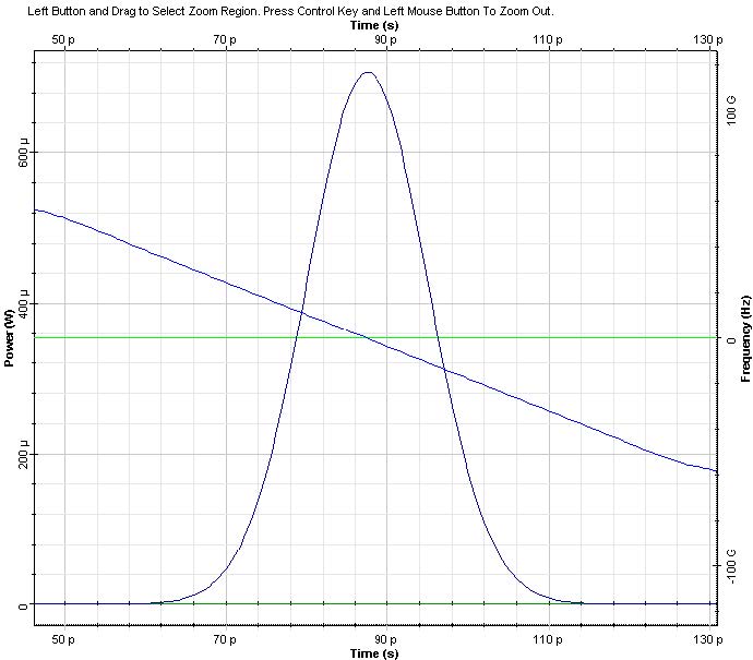
The results for the output pulse shape and chirp are presented in Figure 7. It can be seen that an exact compensation between the dispersion induced and initial chirp occurs, and that the peak power of the pulse is 2.2mW, as given by Equation 9.

OptiFDTD is a powerful, highly integrated, and user friendly CAD environment that enables the design and simulation of advanced passive and non-linear photonic components.

The optimal design of a given optical communication system depends directly on the choice of fiber parameters. OptiFiber uses numerical mode solvers and other models specialized to fibers for calculating dispersion, losses, birefringence, and PMD.

OptiFDTD is a powerful, highly integrated, and user friendly CAD environment that enables the design and simulation of advanced passive and non-linear photonic components.

OptiSystem is a comprehensive software design suite that enables users to plan, test, and simulate optical links in the transmission layer of modern optical networks.

Emerging as a de facto standard over the last decade, OptiGrating has delivered powerful and user friendly design software for modeling integrated and fiber optic devices that incorporate optical gratings.

For example, taking 1.62 for N1 and 1.52 for N2 , we find the NA to be .56. By calculating the arc sine (sin-1) of .56 ( 34 degrees) we determine THE CRITICAL ANGLE.

The pulse broadens monotonically with z if β2C > 0 , however, it goes through initial narrowing when . In the latter case, the pulse width becomes minimum at distance [1]:

Optiwave software can be used in different industries and applications, including Fiber Optic Communication, Sensing, Pharma/Bio, Military & Satcom, Test & Measurement, Fundamental Research, Solar Panels, Components / Devices, etc..

Modal analysis is a pivotal component of modelling optical structures. OptiMode serves as a robust CAD platform for the design and modal analysis of waveguide structures.

The figure above depicts a section of a clad cylindrical fiber showing the core with refractive index of N1 and the clad with index of N2. Also shown is a light ray entering the end of the fiber at angle (A), reflecting from the interface down the fiber. However, if angle A becomes too great, the light will not reflect at the interface, but will leak out the side of the fiber and be lost. This angle, beyond which light cannot be carried in a fiber, is called the CRITICAL ANGLE and may be calculated from the two indices of refraction.

To calculate the Critical Angle, first determine the N.A. (Numerical Aperture).The N.A. of any glass combination may be calculated as follows: (where N1= the index of refraction of the core glass), and N2=(the index of refraction of the cladding glass):

Many people believe that using a low N.A. fiber will “focus” the light from a source. This is not true. A narrow N.A. fiber simply admits less light than a wider N.A. fiber, assuming the source is emitting light at a wide N.A..

Angle A (29 degrees) is the acceptance angle of a N.A. .25 fiber. Angle B (45 degrees) is the incident angle from the bulb. Angle C (83 degrees) is the acceptance angle of a N.A. .66 fiber.

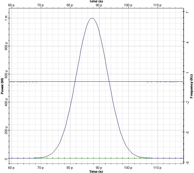
This is shown in Figure 4, where the pulse chirp is plotted together with the pulse intensity. Whereas the input pulse is chirpless, the instantaneous frequency of the output pulse decreases from the leading to the trailing edge of the pulse. The reason for this is GVD. In the case of anomalous GVD (β2 < 0), the higher frequency (“blue-shifted”) components of the pulse travel faster than the lower frequency (or “red-shifted”) ones [1].

The Numerical Aperture is an important parameter of any optical fiber, but one which is frequently misunderstood and overemphasized. In the first illustration above, notice that angle A is shown at both the entrance and exit ends of the fiber. This is because the fiber tends to preserve the angle of incidence during propagation of the light, causing it to exit the fiber at the same angle it entered. Now look at the figure below, which is a drawing of a typical light guide being illuminated by a projector type lamp.

OptiBPM is a comprehensive CAD environment used for the design of complex optical waveguides. Perform guiding, coupling, switching, splitting, multiplexing, and demultiplexing of optical signals in photonic devices.

The equation, which describes the effect of GVD on optical pulse propagation neglecting the losses and nonlinearities, is [1]:

OptiSystem is a comprehensive software design suite that enables users to plan, test, and simulate optical links in the transmission layer of modern optical networks.

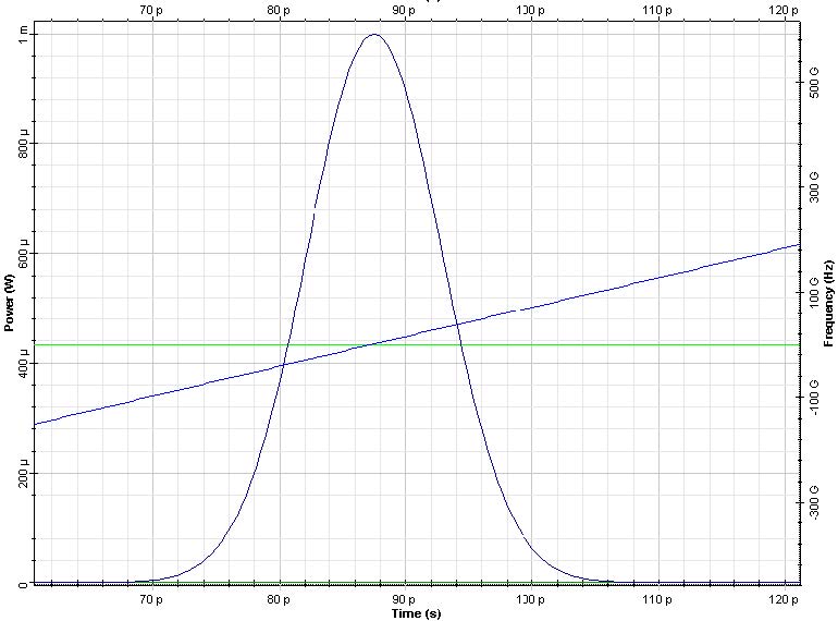
To demonstrate this, we use a chirped Gaussian pulse with the chirp parameter C = 2 (since β2 < 0 in our case) (Figure 6).

Many people believe that using a low N.A. fiber will “focus” the light from a wider N.A. source. This is not true. As you see, the lower N.A. fiber simply has a lower acceptance angle. While the resulting output will be projected into a tighter area, the overall light transmitted is less than what might be transmitted through a higher N.A. fiber. To focus light from a source, a lens assembly must be used to gather all available light and change the incident angle (and resulting N.A.) to match, (or be less than) the N.A. of the fiber being used.

We set the Bit rate equal to 40 Gb/s, which corresponds to bit duration of 25 ps. Using the default value of 0.5 for “width” of the Optical Gaussian Pulse Generator, the resulting FWHM of the pulse is 12.5 ps.

OptiSPICE is the first circuit design software for analysis of integrated circuits including interactions of optical and electronic components. It allows for the design and simulation of opto-electronic circuits at the transistor level, from laser drivers to transimpedance amplifiers, optical interconnects and electronic equalizers.

Additionally, (and somewhat confusing) although the law of physics state the angle of incidence must equal the angle of reflection, life will get in the way when light tavels through longer fibers and fiber bundles. Impurities in glass alter the propagation angle over length such that, if the fiber or fiber bundle is long enough, regardless of input angle, the emitting angle will equal the acceptance angle of the fiber in step index fibers.

Note: The leading edge of the pulse is blue shifted and the trailing edge of the pulse is red-shifted. Because the “blue” and “red” spectral components tend to separate in time, this leads to pulse broadening. However, the pulse spectrum remains unchanged, as Figure 5 shows.

Initial narrowing of the pulse for the case β2C < 0 can be explained by noticing that in this case the frequency modulation (or “chirp”) is such that the faster (“blue” in the case of anomalous GVD) frequency components are in the trailing edge, and the slower (or “red” in the case of anomalous GVD) in the leading edge of the pulse. As the pulse propagates, the faster components will overtake the slower ones, leading to pulse narrowing. At the same time, the dispersion induced chirp will compensate for the initial one. At z = zmin , full compensation between both will occur. With further propagation, the fast and the slow frequency components will tend to separate in time from each other and, consequently, pulse broadening will be observed.

OptiBPM is a comprehensive CAD environment used for the design of complex optical waveguides. Perform guiding, coupling, switching, splitting, multiplexing, and demultiplexing of optical signals in photonic devices.

Manufacturing Standard and Custom fiber optics for Industrial, Medical, Commercial, Military and Machine Vision applications since 1977.

We calculate the project and the obtained results are presented in Figure 3. We see that the pulse is broadened (the peak power decreases in accordance with Equation 4). The origin of pulse broadening can be understood be looking at the instant frequency of the pulse, namely the chirp.