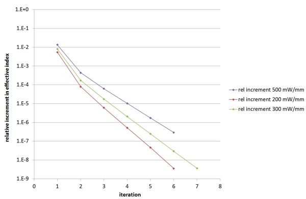
A study of the convergence of the results with the number of iteration is shown below for the different values of input power. The figure of merit plotted vertically is the relative precision on the value of the effective index of the mode. As you can see in the plot below, the changes to the resulting effective index become negligible after just a few iterations.

Kerrlensing

The refractive index of each material and its dependency with temperature was defined via a material database file; in this case the refractive index of each material was set to increases linearly with temperature by 0.01 per degree Celsius. The thermal conductivity of each material was also set.

A heat sink is located at the bottom boundary, all other boundaries are adiabatic. This waveguide was modelled with a substrate thickness of 50um.

Thermallens Camera

You can see below the evolution of the mode profile for the Ex field plotted along a horizontal line in the centre of the GaAs layer when the power in the mode takes values of 0mW/mm (blue), 100mW/mm (purple), 200mW/mm (cyan), 300mW/mm (red) and 500mW/mm (green). You can see that the mode width decreases as the input power increases.

A contour plot of the diffuse heat source can be seen below. The blue regions corresponding to the computational domain used by the optical FDM Solver (optical domain), and the grey regions to additional computational domain used by the Thermal Profiler (thermal domain). The source can be seen near the centre of the optical domain.

Thermal lensingexamples

This simulation was performed on a GaAs/AlGaAs rib waveguide but could be extended to simulate self-heating in any waveguide geometry.

ThermalLens paintball mask

Contour plot of the diffuse source showing the respective size of the computational domains for the optical problem (blue) and thermal problem (grey)

The resulting temperature profile and refractive index profile in the GaAs layer for the “heated waveguide” are shown below for an input power of 100mW/mm.

Unheated waveguide: (top left) cross-section, (top right) refractive index profile at 25ºC, (bottom) mode list displayed in the Mode Finder.

Thermalblooming

In FIMMWAVE’s Thermal Profiler, the intensity profile of the fundamental mode of the “unheated waveguide” was used to define the profile of the heat source. Using this diffuse source and the thermal properties of the “unheated waveguide”, the temperature distribution in the waveguide was calculated by solving the Poisson equation and a first “heated waveguide” was generated, in which the refractive index profile is modified by the temperature distribution.

Thermallens spectroscopy

FIMMWAVE’s Thermo-Optic module can be used to simulate thermal lensing caused by thermo-optic effect in laser cross-sections and optical waveguides. The simulation can be performed very efficiently thanks to the use of distinct computation domain for the thermal and optical problems. The iterative process used in the calculation can be entirely automated using a Python or a MATLAB script.

Introduction Features Applications ‣ SOI Waveguides ‣ Optical Fibres ‣ Photonic Crystal Fibres ‣ Diffused Waveguides ‣ ARROW Waveguides ‣ Slot Waveguides ‣ Bend Modes ‣ Surface Plasmons ‣ Microwave Modes ‣ Thermal Lensing ‣ FIMMPROP applications Options Publications Download Brochure Request evaluation

Thermal lensingapplications

Thermalcamera

This operation was performed for various values of the power in the mode, which allowed us to observe very clearly the thermal lensing effect.

The waveguide was simulated at a wavelength of 1.55um. Its modes were calculated with FIMMWAVE’s FDM Solver, which relies on the finite-difference method.

FIMMWAVE can be used to simulate thermal lensing and self heating effects in optical waveguides and laser diodes using its Thermal Profiler, available as part of the Thermo-Optic module.

Temperature profile of the “heated waveguide” for an input power of 100mW/mm: (right) 3D plot, (left) colour map plot.

The “unheated waveguide” is shown below, along with its refractive index profile and its mode list; the intensity profile of the fundamental TE-like mode is shown in the preview window.

Using distinct computational domains for the optical problem and the thermal problem allows us to optimise computation speed. Indeed, as the temperature varies on a much larger scale than the optical fields it would be very inefficient to solve the optical problem on the same domain as the thermal problem. Different grid resolutions can be used for each solver.

The same process was then started using the mode of the first “heated waveguide” to define the profile of the heat source, and so on iteratively until the results became stable. The whole process was automated using a Python script, which interacted with FIMMWAVE via TCP/IP interface; scripting is also available for MATLAB.