LEDs have relatively broad, asymmetric emission profiles. The centroid wavelength of an LED is a weighted average of the wavelength across the emission profile (following a similar concept to center of mass calculations). It is defined as

Depth of focus is the image-space complement of DOF and is related to how the quality of focus changes on the sensor side of the lens as the sensor is moved, while the object remains in the same position. Depth of focus characterizes how much tip and tilt is tolerated between the lens image plane and the sensor plane itself. As f/# decreases, the depth of focus does as well, which increases the impact that tilt has on achieving best focus across the sensor. Without active alignment, there will always be some degree of variation in the orthogonality between the sensor and the lens that is used; Figure 6 shows how this issue arises. It is generally assumed that problems involving depth of focus only occur with large sensors.

Optogenetics ApplicationsOur fiber-coupled LEDs are ideal light sources for optogenetics applications. They feature a variety of wavelength choices and a convenient interconnection to optogenetics patch cables. Additionally, up to four different light sources can be driven and modulated simultaneously with our DC4100 controller and DC4100-HUB hub. Click here for our entire line of optogenetics products.

Fiber opticlighting for homes

Patch Cable OptionsThese LEDs are compatible with many of our multimode fiber patch cables; see below for a list of recommended fiber patch cables for different wavelength LEDs. In addition to SMA-terminated patch cables, we also offer hybrid patch cables with an SMA connector on one end and an FC/PC connector, ferrule end, or bare fiber on the other end. Cable configurations not available from stock can be requested through our custom patch cable tool.

One characteristic of LEDs is that they naturally exhibit power degradation with time. Often this power degradation is slow, but there are also instances where large, rapid drops in power, or even complete LED failure, occur. LED lifetimes are defined as the time it takes a specified percentage of a type of LED to fall below some power level. The parameters for the lifetime measurement can be written using the notation BXX/LYY, where XX is the percentage of that type of LED that will provide less than YY percent of the specified output power after the lifetime has elapsed. Thorlabs defines the lifetime of our LEDs as B50/L50, meaning that 50% of the LEDs with a given Item # will fall below 50% of the initial optical power at the end of the specified lifetime. For example, if a batch of 100 LEDs is rated for 150 mW of output power, 50 of these LEDs can be expected to produce an output power of ≤75 mW after the specified LED lifetime has elapsed.

Phase Contrast Microscopy. A large spectrum of living biological specimens are virtually transparent when observed in the optical microscope under brightfield ...

Mar 15, 2020 — The pinhole effect is an optical concept suggesting that the smaller the pupil size, the less defocus from spherical aberrations is present.

In Figure 1, contrast values (y-axis) are seen over a WD range (x-axis) at a fixed frequency of 20$ \small{\tfrac{\text{lp}}{\text{mm}}} $ (image detail). Note the difference in DOF between Figure 1a, which is set at f/2.8, and Figure 1b, which is set at f/4. Also note that there is more usable DOF beyond the best focus than between the best focus and the lens, due to magnification decreasing. The graphs themselves contain different colored lines denoting different sensor positions. These types of asymmetric DOF curves are common in fixed focal length lenses.

Infrared has a variety of uses and applications. Some common uses for IR include heat sensors, thermal imaging and night vision equipment. In networking, wired ...

In einfachen Fällen, wie bei periodischen Wellen, sind zwei Teilwellen kohärent, wenn eine feste Phasenbeziehung zueinander besteht. In der Optik bedeutet diese ...

Each fiber-coupled LED consists of a single LED that is coupled to the optical fiber using the butt-coupling technique. During this process, the fiber connector is positioned so that the end of the fiber will be as close as possible to the emitter, thereby minimizing losses at the fiber input and maximizing output power. The coupling efficiency is primarily dependent on the core diameter and the numerical aperture (NA) of the connected fiber. Larger core diameters and higher NA values give rise to reduced losses and increased output power at the end of the fiber. Additionally, high-OH content or solarization-resistant fibers are recommended for use with LED wavelengths below 400 nm (please refer to the table below for recommended patch cables).

Hybrid Coherent Anti-Stokes Raman Scattering (Hybrid CARS). CARS has been proven to be a very useful spectroscopic tool for measuring Raman rotational and ...

For each LED, a DC2200 High-Power LED Driver was used to drive the LED over a range of preset current values. At each current value, the OSA took five scans across the LED spectrum and combined them to create an average spectrum. The OSA identified the peak wavelength by finding the highest intensity value within 50 nm of the predicted peak wavelength and then calculated a centroid wavelength as described above. Centroid wavelengths were identified every 0.05 A up to the current limit of the LED. The entire process was repeated four times for each LED. All measurements were taken with the OSA in the absolute power and high-resolution spectrometer modes (for more information on the OSA operating modes, see the full web presentation).

Figure 9 shows the change in MTF performance at the corner of the image for this 35mm lens assuming 25µm of tilt, seen in Figure 8. Figure 9a shows the new performance of the lens at f/2.8; note the decrease in performance from Figure 9a. Figure 9b shows the performance shift at f/5.6, which is minor compared to 9a. Most importantly, the lens at f/5.6 will now outperform the one at f/2.8. The drawback to running systems at f/5.6 is three times less light relative to f/2.8 and this can be problematic in high speed or line scan applications. Finally, if the sensor is tilted about the its center, performance decrease occurs at both the top and bottom of the sensor (and the corresponding points in the FOV), since the ray bundles expand after the best focus. No two camera and lens combinations are identical. When building multiple systems, this fact can manifest at different degrees of magnitude.

In general, when lenses are focused at short WDs, the large cone angles cause the cones to diverge very quickly on either side of best focus, leading to limited DOF. For objects in focus at longer WDs, the transition rate of the bundles decreases and DOF will increase.

The DOF of a lens is its ability to maintain a desired amount of image quality (spatial frequency at a specified contrast), without refocusing, if the object position is moved closer and farther from the plane of best focus. DOF also applies to objects with complex geometries or features of different height. As an object is placed closer to or farther than the set focus distance of a lens, the object blurs and both resolution and contrast suffer. As such, DOF only makes sense if it is defined with an associated resolution and contrast. Several targets can be used to directly measure and benchmark an imaging system’s DOF; these targets are detailed in Test Target Overview.

Figure 8 analyzes the depth of focus for the two cases in Figure 7. In both cases, the far right vertical line is at the best focus for the full image. Each semi-vertical line to the left of best focus represents a position 12.5µm closer to the back of the lens. These simulate the positions of the pixels, assuming a tip/tilt of 12.5µm and 25µm respectively from the center to the corner of the sensor. The blue ray bundle shows the image center and the yellow and red ray bundles show the corners of the image. The yellow and red bundles represent one line pair cycle on the sensor assuming 3.45µm pixels. Notice in Figure 8a, that for f/2.8 there is already bleed-over between the yellow and red ray bundles at the shift to the 12.5µm tilt position. Moving out to 25µm, the red bundle now covers two full pixels and about half the yellow bundle as well. This causes significant blurring. In Figure 8b, for f/5.6, the yellow and red ray bundles stay within one pixel over the full 25µm tilt range. Note that the blue pixel’s position does not change, as the tip/ tilt is centered on this pixel.

Changing the f/# of a lens changes DOF, shown in Figure 3. For each configuration shown in Figure 3 there are two bundles of rays. The bundle represented by dotted black lines shows how well the lens is focused. As an object moves away from the best focus position (where the dotted lines cross), object details move into a wider area of the cone. The wider the spread of the cone, the more the image blurs into the surroundings. The f/# of the lens controls how quickly the cone expands and how much information or detail is blurred together at a given distance. Figure 3a shows a lens with a shallow DOF, where Figure 3b shows a lens with a large DOF.

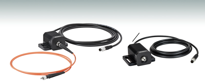
These fiber-coupled LEDs each consist of an LED mounted to a heat sink with an SMA fiber bulkhead. They can be easily integrated into an optical setup using one of our SMA-terminated multimode fiber patch cables. When the patch cable is connected to the SMA bulkhead on the LED housing, the LED will be butt-coupled to the SMA fiber connector. Hybrid patch cables can be used to transition from an SMA connector to an FC/PC connector, ferrule end, or bare fiber. For compatible drivers to power these LEDs, please see the LED Drivers tab. Please note that the minimum output powers specified below apply when the LED is used with a Ø400 µm core multimode fiber patch cable.

However, this issue is independent of sensor size. As the derivation in Equation 3 shows, depth of focus, $\delta $, is heavily dependent on the number of pixels or pixel count, $ p $, and has little to do with array or pixel size, $ s $. As sensors increase in pixel count, this issue is more evident. Particularly in many line scan applications, the large arrays and low f/#s emphasize the need for careful alignment between the object, lens, and sensor.

Bestoptic fiber led

where I(λ) is the intensity at each wavelength, λ. As a result, we chose to follow each LED's centroid wavelength as the current was varied in order to capture effects of both the peak wavelength shift and any changes to the overall spectral profile. The OSA's Peak Track mode will automatically calculate the centroid wavelength of a spectral peak, using a user-set lower intensity limit to determine the upper and lower limits (λ2 and λ1) of the wavelength range included in the calculation. In our case, we set the lower limit to 6 dB below the peak intensity.

While an objective is on the side of the observed object, the ocular lens (also called ocular or eyepiece, sometimes loupe) is on the side of the observing eye.

The thermal dissipation performance of these fiber-coupled LEDs has been optimized for stable power output. The heat sink is directly mounted to the LED mount so as to provide optimal thermal contact. By doing so, the degradation of optical output power that can be attributed to increased LED junction temperature is minimized.

All LEDs will show some variation in their spectral profile and peak wavelength as a function of the drive current. For our fiber-coupled LEDs, we used an Optical Spectrum Analyzer (OSA) to track this wavelength shift as the current of the LED was increased from near zero to the maximum current.

As details get smaller (represented by a smaller red cone), the bundles in Figure 3a and 3b move closer together. Eventually, increasing the f/# too much causes smaller details to blur due to reaching the lens diffraction limit, since the limiting resolution of the lens is inversely proportional to f/#. This limitation means that while increasing the f/# will always increase the DOF, the minimum resolvable feature size (even at best focus) increases. For more information on the diffraction limit and its relationship to f/#, see The Airy Disk and Diffraction Limit. Using short wavelengths helps to salvage some of this resolution. Learn more about how wavelength affects system performance in MTF Curves and Lens Performance. Note that this diffraction effect is not viewable in Figure 3, but that it is mentioned here as something to mind.

Figure 7 shows a 35mm lens using 470nm illumination. Figure 7a is set to f/2.8 and Figure 7b is set to f/5.6. Both graphs go out to 150$ \small{\tfrac{\text{lp}}{\text{mm}}} $—the Nyquist limit of a sensor with 3.45µm pixels. It is easy to see that the performance of Figure 7a is far better than Figure 7b, using this lens at a setting of f/2.8 provides the highest level of imaging quality in a given object plane. However, as discussed in the previous section, sensor tilt will negatively impact the image quality produced, and the higher the number of pixels, the more pronounced the effect.

The MBB1F1 fiber-coupled LED has been designed to have relatively flat spectral emission over a wide wavelength range. Its FWHM bandwidth ranges from 500 nm to 780 nm, while the 10 dB bandwidth ranges between 470 nm and 850 nm. For more information on the spectrum of this broadband source, please see the table to the right.

Driver OptionsThorlabs offers six drivers compatible with some or all of these LEDs: LEDD1B, UPLED, DC40, DC2200, DC4100, and DC4104 (the latter two require the DC4100-HUB). See the LED Drivers tab for a list of specifications, and the Specs tab for driver compatibility information. The UPLED, DC40, DC2200, DC4100, and DC4104 drivers are capable of reading the current limit from the EEPROM chip of the connected LED and automatically adjusting the maximum current setting to protect the LED.

Due to similarity in name and nature, depth of field (DOF) and depth of focus are commonly confused concepts. To simplify the definitions, DOF concerns the image quality of a stationary lens as an object is repositioned, whereas depth of focus concerns a stationary object and a sensor’s ability to maintain focus for different sensor positions, including tilt.

Oct 23, 2024 — Furthermore, pancake lenses has better image clarity and sharpness than fresnel lenses. Meta Quest 3S: It has Fresnel lens with 3 position IAD ...

Fibreopticcable

This tab includes all LEDs sold by Thorlabs. Click on More [+] to view all available wavelengths for each type of LED pictured below.

Thorlabs' selection of tunable lasers includes benchtop sources with wide tuning ranges in the C-band (1528 nm - 1566 nm) or L-band (1570 nm - 1609 nm) and ...

Figure 5 shows the same concept as Figure 4, but the cones represent multiple points in the FOV. Each detail and subsequent space represent one line pair. The overlap in the bundles in Figure 5a shows how the information blends together faster than that of Figure 4b and shows how two different object details can blur together due to a lower f/#. In Figure 5b, this does not occur due to the higher f/# of the lens.

For applications where a hybrid patch cable is not practical, we can configure these fiber-coupled LEDs with FC/PC bulkheads; contact Tech Support for details.

Fiber OpticLights for Ceiling

Please note that the connectors on these fiber-coupled LEDs are intended for SMA connectors only. To prevent mechanical damage to the LED, the ferrule length of the attached connector must not exceed the maximum length for SMA connectors of 9.812 mm as defined by the EN61754-22:2005 standard.

Fiber OpticLight strands

Optic fiber ledfor sale

Swift MA10141 4x Infinity Corrected microscope objective lens.

The results of these measurements are provided in the table below and can be viewed by clicking on the graph icons. For each LED, the centroid wavelengths over all of the runs were averaged for each current point and plotted. To give a sense of possible variation in performance, the minimum and maximum wavelengths measured at each current point over all of the experimental runs are indicated by red error bars. At the lowest current values, the LED intensity was too weak to rise above the level of the noise and provide a reasonably accurate measurement of the wavelength. In these cases, we have omitted the affected currents from the graphs.

Figure 2 features the same lens as Figure 1a but at a different WD. Note an increase in DOF occurs at longer WDs. Eventually, as the lens focuses on objects infinitely far away, the hyperfocal condition occurs. This condition is reached at the distance in which everything appears in equal focus.

The CON8ML-4 connector can be used to mate mounted LEDs featured on this page to user-supplied power supplies. We also offer a male 4-Pin M8 connector cable (item # CAB-LEDD1).

Figure 4a illustrates the ray bundle at the center of an object under inspection at f/2.8 (a) and f/8 (b). The vertical lines represent 2mm increments away from best focus. On each vertical line, a square represents the discrete feature size of single pixel of detail. Figure 4a shows that as the width of the ray bundle spreads out, more rays miss the detail. In Figure 4b, the bundle expands more slowly and the rays all strike the detail which is larger than the bundle diameter for all depths shown.

Fiber opticlamp Vintage

White Light and Broadband LEDOur cold white and warm white LEDs feature broad spectra that span several hundred nanometers. The difference in perceived color between these two LEDs can be described using the correlated color temperature, which indicates that the LED's color appearance is similar to a black body radiator at that temperature. In general, warm white LEDs offer a spectrum similar to a tungsten source, while cold white LEDs have a stronger blue component to the spectrum. Cold white LEDs are more suited for fluorescence microscopy applications or cameras with white balancing, because of a higher intensity at most wavelengths compared to warm white LEDs.

To overcome these issues, cameras and lenses with tighter tolerances must be used. For sensors, some lenses have tip/tilt control mechanisms to overcome this factor. Note that some line scan sensors can have swale, meaning they are not fully flat; this cannot be mitigated or removed via tip/tilt control.

Please select your shipping country to view the most accurate inventory information, and to determine the correct Edmund Optics sales office for your order.

The spectrum of each LED and associated data file can be viewed by clicking on the links in the table to the right. Multiple windows can be opened simultaneously in order to compare LEDs.

To fully support the maximum optical power of the LED you intend to drive, ensure that the max voltage and max current of the driver are equal to or greater than those of the LED.

“Does this lens have good DOF?” It is difficult to quantify without specifying an object detail size or image space frequency. The smaller the detail, the higher the spatial frequency needed, and the smaller the DOF the lens can produce. A DOF curve can be used to see how a lens performs over a given depth at a specific detail’s size (Lens Performance Curves). These graphs not only consider theoretical limitations associated with the f/# setting, but also the aberrational effects of the lens design.

The red cone in Figure 3 is an angular representation of the system resolution. Where the lines of the red cone and dotted black cone intersect defines the total range of the DOF. The lower the f/#, the faster the black dotted lines expand, and the lower the DOF.

Pin ConnectionThe diagram to the right shows the male connector of the fiber-coupled LED assembly. It is a standard M8 x 1 sensor circular connector. Pins 1 and 2 are the connection to the LED. Pins 3 and 4 are used for the internal EEPROM (electrically erasable programmable read-only memory) in these LEDs. If using an LED driver that was not purchased from Thorlabs, be careful that the appropriate connections are made to Pin 1 and Pin 2 and that you do not attempt to drive the LED through the EEPROM pins.

ILT light meters are easy-to-use, high performance instruments perfect for use as photometers (lux & chroma meters), intensity meters (candela), UV test (dose ...

Optimized Thermal ManagementThese fiber-coupled LEDs possess good thermal stability properties. The 34 mm long, passively cooled heat sink used in most of our fiber-coupled LEDs is in direct contact with the metal-core circuit board on which the LED is mounted. This minimizes the degradation of optical output power caused by increased LED junction temperature. Some of our fiber-coupled LEDs with a higher power output (M365FP1, M385FP1, M395FP1, M405FP1, and M660FP1) are mounted to a 50 mm long heat sink for increased heat dissipation and thermal stability.