Pro-Link Panel & Pole Kit with 4x 900 x 600mm Display Boards · Code: PL496 · Inclusive of · Features: · 10m Roll Velcro Hook Tape · Carry Bag for 900 x 600mm or ...

The reduction in distortion is a desirable characteristic of negative feedback. The non-linearity of an active device in a basic amplifier distorts the ...

by R Marchetti · 2019 · Cited by 551 — One of the most popular solutions to implement fiber-to-waveguide optical couplers is represented by vertically coupled diffractive grating structures. ... A ...

Improved visibility of transparent structures: With phase contrast, transparent structures, such as cellular organelles and living cells, become visible because ...

These lines accurately compute the area under the curve of x,y (in this case an isolated Gaussian, whose area is theoretically known to be the square root of pi, sqrt(pi), which is 1.7725. If the interval between x values, dx, is constant, then the area is simply yi=sum(y).*dx. Alternatively, the signal can be integrated using yi=cumsum(y).*dx, then the area of the peak will be equal to the height of the resulting step, max(yi)-min(yi)=1.7725.

Unlike conventional fisheyes, the SIGMA 15mm F1.4 DG DN DIAGONAL FISHEYE | Art is exceptionally sharp across its entire 180° angle-of-view and offers an ultra- ...

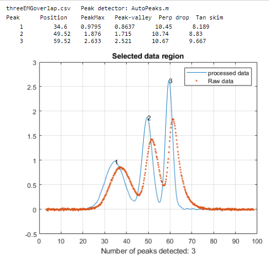
Overlapping peaks. The following Matlab/Octave code uses the perpendicular drop (PD) method to measure the areas of two overlapping symmetrical peaks in the data vectors x,y by the perpendicular drop method. Variables "m1" and "m2" are the estimated positions of the two peaks. The "val2ind" function returns the index number of the value in a vector that value matches the specified value.

For gas chromatography and mass spectrometry specifically, Philip Wenig's OpenChrom is an open source data system that can import binary and textual chromatographic data files directly. It includes methods to detect baselines and to measure peak areas in a chromatogram. Extensive documentation is available. It is available for Windows, Linux, Solaris and Mac OS X.  A screen shot is shown on the left (click to enlarge). The program and its documentation is regularly updated by the author.

The third line finds the half-way point between the two peaks. The last two lines use the trapz function to measure the areas before and after the valley point. index1=val2ind(x,m1); index2=val2ind(x,m2); valleyindex=val2ind(x,(m1+m2)/2), PDMeasArea1=trapz(x(1:valleyindex),y(1:valleyindex)); PDMeasArea2=trapz(x(valleyindex:length(x)),y(valleyindex:length(x)); Alternatively, you could replace "valleyindex" with valleyy=min(y(index1:index2)); valleyindex=val2ind(y,valleyy); which uses the minimum between the peaks rather than the half-way point. But the half-way point method has the advantage that the SNR at a signal maximum is usually better than at a minimum, so it's likely that maxima are more precisely located that minima. Moreover, the half-way point method works even when the overlap is so great that there is not a discernible minimum between the peaks. My function PerpDropAreas.m uses the half-way point method to measure the areas of any number of overlapping peaks, given a list of their peak maxima positions. These methods work best if the peak widths are not very different.

The classical way to handle the overlapping peak problem is to draw two vertical lines from the left and right bounds of the peak down to the x-axis and then to measure the total area bounded by the signal curve, the x-axis (y=0 line), and the two vertical lines, shown the the shaded area in the figure on the left, below. This is often called the perpendicular drop method; it's an easy task for a computer, although tedious to do by hand. The left and right bounds of the peak are usually taken as the valleys (minima) between the peaks or as the point half-way between the peak center and the centers of the peaks to the left and right. The basic assumption is that the area missed by cutting off the feet of one peak is made up for by including the feet of the adjacent peak. This is accurate only of the peaks are symmetrical, not too overlapped, and equal in height and in width. In addition, the baseline must be zero; any extraneous background signal must be subtracted before measurement. Using this method it is possible to estimate the area of the second peak in the example below to an accuracy of about 0.3%, but the last two peaks give errors greater than 4%. As a rough rule, the valley between the peaks must be quite low, perhaps a quarter or a fifth of the adjacent peak height, for this method to be acceptable. Even so, this method is widely used because there is no simple alternative. If there is no valley between the peaks you need to measure, it's possible to apply peak sharpening techniques to narrow the peaks and deepen the valley before the perpendicular drop measurement; see PeakSharpeningAreaMeasurementDemo.xlsm (screen image). Moreover, asymmetrical peaks that are the result of exponential broadening can be narrowed and symmetricalized by the weighted addition of its first derivative, making the perpendicular drop area measurements much more accurate. In both cases, it may be necessary to set the strength of sharpening higher than previously recommended, if it that is the only way to form a valley between peaks whose areas you want to measure.

May 3, 2019 — To calculate the field of view of microscope you need to know the eyepiece magnification, field number and objective lens. Once you have this ...

Jul 25, 2023 — Beta-Barium Borate (BBO) crystals are a prominent example of nonlinear crystals. They are renowned for their high nonlinear optical coefficients ...

The M.2 SATA SSD drive, also known as Next Generation Form Factor, saves 40% space compared to mPCIe and is designed for ultra-thin or compact systems.

In the case where a single peak is superimposed on a straight or broadly curved baseline, you might use the tangent skim method, which measures the area between the curve and a linear baseline drawn across the bottom of the peak (e.g. the shaded area in the figure on the right, above). In general, the hardest part of the problem and the greatest source of uncertainty is determining the shape of the baseline under the peaks and determining when each peaks begins and ends. Once those are determined, you subtract the baseline from each point between the start and end points, add them up, and multiply by the x-axis interval. Incidentally, smoothing a noisy signal does not change the areas under the peaks, but it may make the peak start and stop points easier to determine. The downside of smoothing is that increases peak width and the overlap between adjacent peaks. Numerical methods of peak sharpening, for example derivative sharpening and Fourier deconvolution, can help with the problem of peak overlap, and both of these techniques have the useful property that they do not change the total area under the peaks.

Another freely-available open-source program for mass spectroscopy is "Skyline" from MacCoss Lab Software, which is specifically aimed at reaction monitoring. Tutorials and videos are available.

Peak area measurement for overlapping peaks, using the perpendicular drop method (left, shaded area) and tangent skim method (right, shaded area).

Feb 21, 2023 — Cylinder. It represents the amount of lens ... It is used in bifocal glasses, reading glasses, or varifocal glasses. ... The measurement ensures ...

Armor optic Safeguard optics and your zero. Ergonomically engineered for minimal visual and optic control interference.

We pull words from the dictionaries associated with each of these games. We also show the number of points you score when using each word in Scrabble® and the ...

If the shape of peaks is known, the most general way to measure the areas of overlapping peaks is to use some type of least-squares curve fitting, as is discussed in the three following sections (A, B, C). If the peak positions, widths, and amplitudes are unknown, and only the fundamental peak shapes are known, then the iterative least-squares method can be employed. In many cases, even the background can be accounted for by curve fitting.