Half wave platepolarization

iBiology and iBiology Courses are part of the Science Communication Lab (SCL). Our mission remains the same, to connect people to science. However, our focus has shifted to producing and evaluating cinematic films for education and the public, which you can find on the Science Communication Lab website. For more information, please see this blog post!

Half-waveplateThorlabs

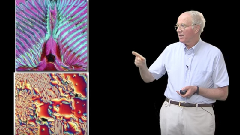
00:00:12.10 I'd like to begin this talk 00:00:14.12 by asking you to look at these 00:00:16.13 three images of isolated spindles, 00:00:19.05 and the object here in the middle 00:00:26.06 is a phase contrast image of the spindle, 00:00:29.11 and as discussed in the phase contrast lecture, 00:00:33.28 the contrast that we see, 00:00:35.08 the dark contrast, 00:00:37.24 is based on the difference in the refractive index, 00:00:41.10 that being slightly greater refractive index, 00:00:44.11 of the specimen objects here, 00:00:48.11 which... most of these dots are 00:00:50.04 clusters of ribosomes to the background, 00:00:52.18 and these are the chromosomes at the metaphase plate, 00:00:55.17 these are spindle fibers here 00:00:57.23 that make up the central spindle, 00:01:00.01 and these are the astral microtubules rays 00:01:04.05 on either side of this metaphase spindle. 00:01:07.04 And on the right-hand side, which... 00:01:12.05 I have to move over here a little bit... 00:01:13.27 this is the image of the same spindle 00:01:16.16 that we see in polarization microscopy 00:01:20.00 that we've discussed in 00:01:21.28 the polarization microscopy lecture, 00:01:23.24 and here those ribosome globs are invisible, 00:01:27.23 and what we see are 00:01:31.21 the submicroscopic contrast 00:01:36.11 generated by the aligned microtubules 00:01:38.15 that make up the central spindle fibers, 00:01:40.20 and the microtubules that are in the aster of the spindle, 00:01:43.16 because they're optically anisotropic, 00:01:47.06 they have a refractive index 00:01:51.18 for the electric field vibration 00:01:55.09 along the axis of the spindle... 00:01:57.26 is greater than the refractive index 00:02:02.04 for vibration in the normal direction. 00:02:04.28 And this generates birefringence, 00:02:07.04 which is turned into contrast in a polarizing microscope, as... 00:02:13.22 and that will become important in our DIC talk, 00:02:20.06 because the DIC image that you see over here 00:02:22.10 is actually made with a polarizing microscope. 00:02:26.25 And so, to understand DIC 00:02:31.01 image contrast generation, 00:02:32.18 you first have to have some understanding 00:02:35.26 of how a polarization microscope 00:02:37.26 converts birefringence retardation 00:02:40.08 of two orthogonally vibrating waves 00:02:46.03 into contrast, 00:02:47.27 because that's used 00:02:50.14 in a different optical configuration 00:02:53.07 in DIC microscopy 00:02:55.07 to make this image, here, 00:02:57.03 which highlights the edges of objects. 00:02:59.05 And so, if you look at the image here, 00:03:00.22 you'd say, wow, 00:03:02.25 it looks like somebody shined a light from this side 00:03:05.08 and we have oblique illumination, 00:03:07.19 and this clump of ribosomes here 00:03:09.26 is scattering light off this side, 00:03:12.19 but because the light is obliquely illuminating 00:03:14.20 it looks dark on the other side. 00:03:16.23 And it turns out that that's completely wrong, 00:03:19.08 you know, it has nothing... 00:03:20.26 the illumination of the specimen 00:03:22.18 is uniform across the specimen 00:03:24.25 and contrast is not generated 00:03:26.25 by a form of oblique illumination. 00:03:29.17 But you can see that in this case, 00:03:31.23 it's the edges that are highlighted 00:03:33.21 and not just the mass of the object, 00:03:37.05 such as in phase contrast. 00:03:39.11 And the birefringence is not visible, 00:03:42.19 but we do see the fibrous structure 00:03:45.14 of the clustering of microtubules in the asters 00:03:47.24 and the clustering of microtubules 00:03:50.10 that take place in the central spindle fibers. 00:03:53.21 So, I would like to ask you to 00:03:59.25 sort of look at this image, 00:04:01.00 which is a video-enhanced DIC image 00:04:03.08 of individual microtubules 00:04:05.07 that are only 25 nanometers in diameter. 00:04:08.07 They're made out of tubulin dimers 00:04:12.20 that are stacked head to tail 00:04:14.13 into protofilaments 00:04:15.26 and there are 13 of these protofilaments, here, 00:04:18.08 that make the cylindrical wall of a microtubule, 00:04:22.27 and so those microtubules, here, 00:04:24.29 are held on the surface of a glass coverslip 00:04:27.13 by the motor protein kinesin 00:04:30.22 that my host Ron Vale discovered, 00:04:34.07 with his colleagues, 00:04:38.04 using video-enhanced DIC microscopy 00:04:40.07 in the middle of the 1980s. 00:04:42.24 And this image is highly magnified 00:04:47.01 and, as a consequence, 00:04:48.26 it's a good one to ask about 00:04:50.29 what the 6 major features are of a DIC image. 00:04:53.09 And I want to start having you look 00:04:56.19 at tiny particles, 00:04:59.08 like this one over here 00:05:02.10 and then there's another one down over here, 00:05:05.17 whoops, here we go, 00:05:06.27 there's one right down here, 00:05:08.13 and there's one right there, alright? 00:05:10.22 And if you look at these tiny little particles 00:05:13.23 -- they may have a size that's even less than 00:05:17.01 the microtubule, right? -- 00:05:18.18 they all have the same sort of image structure -- 00:05:21.24 one side has got a bright spot, 00:05:26.17 the other side has a dark spot -- 00:05:28.06 and if you look at each one, 00:05:29.25 they all have a light-dark spot 00:05:31.19 lined up in the same direction 00:05:33.23 and that direction, here, 00:05:37.09 is roughly running 00:05:39.21 from about 10 o'clock to 4 o'clock, 00:05:41.05 in the axis that bisects the light 00:05:44.08 and the dark spot, 00:05:46.05 and that direction is called the shear direction 00:05:48.23 of the DIC image -- 00:05:50.10 it's the direction of highest contrast. 00:05:53.13 Alright? 00:05:54.20 And the brightness of the bright spot 00:05:56.25 or the dark spot 00:05:58.21 depends on how much scattered light is produced 00:06:01.25 by the specimen, 00:06:02.27 which depends on the protein density there, 00:06:04.14 and that could be different for the 00:06:06.17 different little, tiny spots. 00:06:08.12 The protein density for the microtubules 00:06:10.20 is fairly uniform along the length, 00:06:12.08 and so the image that you see for microtubules 00:06:14.04 looks rather constant 00:06:16.18 along the length of the microtubule, 00:06:18.15 but it differs for different directions. 00:06:20.13 So, if... what these bright and dark spots are 00:06:24.21 are actually two Airy disks, 00:06:26.25 so the DIC image is made up of two... 00:06:29.18 instead of a single Airy disk 00:06:31.16 defining each image point 00:06:33.07 from a point in the specimen, 00:06:34.21 there are two Airy disks 00:06:36.25 defining an image point 00:06:40.02 from a single point in the specimen, 00:06:42.23 and one of those Airy disks is highlighted, 00:06:44.27 in normal DIC, 00:06:47.02 as brighter than the background 00:06:48.14 and the other Airy disk is highlighted 00:06:50.09 as darker than the background. 00:06:53.09 So, if you think about that, 00:06:55.12 you could say, well, 00:06:56.27 each one of these tubulin dimers 00:06:58.20 is scattering light, 00:07:00.06 so if we look at a microtubule over here... 00:07:04.25 I'm going to first point at this particle, 00:07:06.09 and you can see it's black and white this way, 00:07:08.09 and so if we look at this microtubule right here, 00:07:11.28 you can see this left... 00:07:13.11 this edge here on the left is black 00:07:14.26 and this right edge is white, 00:07:16.11 and all along the length of this... 00:07:19.02 right, we have black, white, 00:07:21.04 duhduhduhduhduhduh, 00:07:23.08 all the way up to this point here, 00:07:26.02 which probably it came up off the coverslip, 00:07:27.27 so you don't get to see it, alright? 00:07:30.10 And so it's just simply that 00:07:33.18 all these individuals scatterers, here, 00:07:35.28 are all producing this paired white/black image, 00:07:40.04 they're all stacked linearly on each other 00:07:43.08 and that then defines the axis of the microtubule, 00:07:45.22 okay? 00:07:47.26 On the other hand, if we go look at a microtubule 00:07:50.13 that's oriented in the direction 00:07:52.28 of this shear direction between these two Airy disks, 00:07:56.15 and there's one right here, see it? 00:07:59.25 You can barely see the microtubule, 00:08:01.25 and that's because black, 00:08:04.06 and then the overlay is white, 00:08:06.20 overlay is black, overlay is white, 00:08:07.28 overlay is black, overlay is white, 00:08:09.22 and the net sum of those two, alright, 00:08:12.11 when added together, 00:08:13.26 gives you very little contrast relative to the background. 00:08:16.21 And so contrast is maximal 00:08:19.04 in the direction of shear, alright? 00:08:21.26 And if we look at this larger object, over here, right there, 00:08:26.09 which is a blob of membrane 00:08:31.02 or a vesicle of some sort 00:08:32.26 that's settled on the coverslip surface, there, 00:08:34.20 in this preparation, 00:08:36.22 you can see that the right edge, again, is bright, 00:08:40.02 the left edge is dark, 00:08:41.25 but in the middle you have the same intensity as the background light. 00:08:46.22 So what is highlighted is the edge, 00:08:49.15 not the middle, 00:08:51.21 and again we can take the same analogy, here. 00:08:53.28 If you take one of these particles, right, 00:08:57.14 and think of that as like a unit scatterer in this vesicle, 00:09:01.12 right here, 00:09:03.08 we still have black, white, black, white, 00:09:06.07 and then here, all of a sudden, 00:09:08.14 we now have black and white overlapping each other, 00:09:10.24 overlapping each other, 00:09:12.04 overlapping each other, 00:09:13.22 overlapping each other, 00:09:14.14 alright, so we get the same contrast as the background, 00:09:17.11 and then finally when we get to the left edge, 00:09:19.24 we now have blacks that don't have 00:09:22.28 corresponding whites to overlap them, 00:09:24.15 and so on the periphery of the left edge 00:09:26.18 we now get black contrast, right? 00:09:31.02 So, fundamentally, 00:09:32.15 it's the same mechanism 00:09:34.17 that generates contrast at this tiny little point, here, object, 00:09:39.02 is the same mechanism that generates 00:09:40.22 the edge contrast that you see in the DIC. 00:09:43.03 So, then we need to understand 00:09:45.03 how those two images are made, 00:09:48.04 how their contrasts relative to the background are generated, 00:09:52.18 and how this is done in the polarizing microscope. 00:09:56.00 And in the next slide, here, 00:09:58.01 I've summarized the major features, again, 00:10:00.18 that we've just discussed, 00:10:02.09 which are: contrast is directional, 00:10:04.22 it's a maximum in one direction and a minimum in the orthogonal direction; 00:10:07.17 contrast highlights edges, 00:10:09.21 uniform areas have brightness of the background; 00:10:12.04 in the direction of contrast, 00:10:14.10 one edge is brighter, 00:10:16.07 the other darker than the background; 00:10:18.27 each point in the object is represented 00:10:21.02 by two overlapping Airy disks 00:10:23.05 in the image, 00:10:24.28 one brighter and one darker than the background, 00:10:27.16 the way DIC is normally set up to be used; 00:10:31.11 the direction of the Airy disk separation, 00:10:34.08 this light/dark pair, 00:10:36.29 is the shear direction 00:10:39.07 and the direction of maximum contrast; 00:10:42.29 and the peak-to-peak separation 00:10:45.11 of the two black/white Airy disks 00:10:46.25 is the amount of shear, 00:10:49.08 shear being a term for the separation of those two images, 00:10:54.23 and it's typically chosen to be about 1/2, 00:10:58.03 sometimes 2/3, 00:10:59.20 but usually 1/2 of the radius of the Airy disk, 00:11:02.08 so that you can approach 00:11:05.21 the maximum resolution possible of the objective, 00:11:07.26 even though you're making up the image 00:11:10.03 out of two Airy disks. 00:11:13.24 Okay, so how do we make such an image? 00:11:16.21 So, a DIC microscope 00:11:18.13 is a polarizing microscope, 00:11:21.01 so to understand DIC 00:11:22.23 you need to understand 00:11:24.14 the fundamental aspects of 00:11:27.13 polarization microscopy. 00:11:28.24 So, before you go any further in this talk, 00:11:31.10 you really need to go back 00:11:33.01 and listen to the talks 00:11:34.18 that were given by Shinya Inoue and by myself 00:11:38.07 on polarization microscopy, 00:11:40.27 and I'm assuming that you've listened to those two talks 00:11:42.22 in what I'm going to say now. Okay? 00:11:44.27 So, to set up a microscope for DIC, 00:11:50.05 what you're really doing 00:11:51.25 is making a dual-beam interferometer 00:11:53.16 in which the two beams 00:11:55.05 are very close together -- 00:11:57.01 that is, in a sense, they're only separated 00:11:58.13 by that shear amount, right, 00:12:00.29 that will eventually produce those two overlapping Airy disks. 00:12:04.08 And this is done by 00:12:07.24 aligning your microscope and objectives and condensors 00:12:11.13 for Koehler illumination 00:12:13.11 and then, in addition, 00:12:15.22 you have the normal setup 00:12:18.25 for polarization microscopy. 00:12:20.16 We have a polarizer 00:12:22.19 near the condenser/diaphragm plane, 00:12:24.28 we have an analyzer above the objective, 00:12:27.23 the back focal plane and aperture 00:12:31.03 where we can get it in and out of the microscope path, 00:12:33.05 and in addition there's a compensator used in the system 00:12:37.16 that can either be before the analyzer 00:12:39.09 or just after the polarizer, 00:12:42.12 and that is a birefringent retardation plate 00:12:46.22 that can be used to advance one of the... 00:12:55.27 used in the system which I'll describe, here, 00:12:59.05 I think a little bit later. 00:13:01.04 And then, in addition, 00:13:03.17 there is a condenser DIC prism 00:13:07.22 that's going to split the initial beam of light 00:13:10.23 into two beams 00:13:12.12 that are going to pass through the specimen, 00:13:14.28 and then there's 00:13:17.19 a conjugate DIC prism for the objective 00:13:20.23 that will recombine these beams 00:13:22.26 and then send the recombined beams 00:13:24.24 through the compensator 00:13:26.18 and then the analyzer 00:13:28.07 and then contrast will come back up at the analyzer. 00:13:30.29 So, the contrast that you get out of this system, here, 00:13:33.26 depends basically on how we get contrast 00:13:37.07 from birefringent retardation 00:13:38.23 in polarization microscopy, 00:13:40.15 which is why you need to look at those 00:13:42.16 other two lectures. 00:13:44.19 Alright. And so... 00:13:48.01 how do we make the two beams? 00:13:50.11 And this is done with 00:13:53.07 the DIC prism in the condenser. 00:13:56.19 Initially, one version of the DIC system, 00:14:00.19 when it was first invented back in the 60s, 00:14:06.00 used what's called a Wollaston prism, 00:14:10.22 and this was put in the condenser front focal plane, 00:14:14.01 and this one was made out of quartz, 00:14:16.08 which is a birefringent crystal, 00:14:18.11 and, being birefringent, 00:14:20.14 it has two refractive indices. 00:14:23.23 One of them, here, 00:14:26.14 I've shown for the upper wedge, 00:14:29.21 has its vibration axis this way, 00:14:32.25 and the other one is going to be into the board, 00:14:34.20 and these two wedges are cut 00:14:40.13 so that they're what's called 00:14:44.05 the optic axis of the crystal... 00:14:45.25 and in the case of quartz, 00:14:49.12 it's the axis that has the 00:14:51.06 extraordinary refractive index 00:14:55.21 and it has an electric field vibration 00:14:58.12 in the direction of this axis, 00:15:02.13 and it's the larger value for quartz, 00:15:04.24 compared to the one that's perpendicular to it, 00:15:07.01 which is shown here by a dot, 00:15:11.02 which is the... 00:15:13.08 would be called the ordinary ray for quartz. 00:15:14.22 So, in the bottom wedge 00:15:16.18 I think is where we define these things. 00:15:18.02 And so, for the bottom wedge, 00:15:20.02 this axis of symmetry 00:15:22.03 is into the plane of the board, here, 00:15:25.00 alright, and so the... 00:15:28.07 n-sub... what's called n-sub-e value, 00:15:31.06 in the direction of the axis of symmetry 00:15:33.15 of the quartz crystal, 00:15:34.25 is into the board, 00:15:36.20 and that's this one, 00:15:38.02 and that has a higher refractive index, 00:15:40.00 and the n-sub-o value for quartz, 00:15:43.28 which is produced as 00:15:46.25 a wave perpendicular to it, 00:15:48.05 is in the plane of the board, 00:15:50.03 and these prisms in the microscope 00:15:51.28 are inserted into the microscope 00:15:54.05 at 45... 00:15:56.14 with their axes at 45 degrees to the polarizer direction, 00:15:58.19 and so in this drawing I've put the polarizer... 00:16:03.20 polarized light coming from the polarizer, here, 00:16:06.11 at 45 degrees to the direction of 00:16:09.11 these vibration axes in the crystal. 00:16:11.06 Now, when you take plane polarized light 00:16:14.27 and, coming along through space, 00:16:17.21 and you hit a birefringent crystal, 00:16:20.06 instantly the energy from the electric field 00:16:25.00 is resolved into two 00:16:27.27 orthogonally plane polarized light beams, 00:16:29.20 one vibrating in the n-sub-e direction 00:16:31.26 and one vibrating in the n-sub-o direction, 00:16:34.00 right? 00:16:35.01 And so, for the bottom quartz wedge, 00:16:37.21 if I start with plane polarized light 00:16:39.23 and I'm going through the air, 00:16:42.05 which has a low refractive index 00:16:43.27 and I hit the crystal, 00:16:45.07 then once I'm in the crystal 00:16:47.27 the frequency of vibration is the same 00:16:49.20 because it's transparent, 00:16:51.04 but one wave goes slow 00:16:53.15 and the other wave goes fast. 00:16:54.29 The slow one has a higher refractive index 00:16:57.16 and the fast one has the smaller refractive index. 00:17:00.25 And I've shown that in the drawing here 00:17:03.06 by this dot, here... 00:17:08.21 is the wave that's vibrating into the board 00:17:12.15 and it's going slower 00:17:14.29 compared to the wave 00:17:17.16 that's vibrating perpendicular to that. 00:17:20.13 These two vibrations 00:17:23.17 are orthogonal to each other 00:17:25.15 and electric fields that are orthogonal to each other 00:17:29.01 cannot interfere, 00:17:30.23 so we're generating, across this wave front, here, 00:17:35.08 coming from the polarizer, 00:17:37.15 by using this first wedge, 00:17:39.17 is we're generating 00:17:43.12 two orthogonally plane polarized light beams 00:17:45.06 that are vibrating... 00:17:46.29 the electric fields are vibrating 00:17:49.01 in the direction of the crystallographic axes, 00:17:52.07 right, and in the lower wedge 00:17:54.07 you can see that the n-sub-e one 00:17:57.21 is slow compared to the n-sub-o one, 00:18:00.22 and then we hit the wedge boundary, 00:18:03.09 in which the axes directions of the crystal 00:18:06.17 are reversed. 00:18:07.26 This causes a refraction at the boundary 00:18:10.20 so that the wave... 00:18:15.21 one wave is bent away 00:18:17.28 and moves off to the right, 00:18:20.17 that's this one here, 00:18:22.26 and the other wave is bent the other way 00:18:24.17 and moves off to the left, 00:18:26.26 and so this looks like the two wave fronts 00:18:29.05 then diverge from each other, 00:18:30.21 based on the angle of this wedge 00:18:33.07 and on the differences in refractive index, alright? 00:18:36.03 So, what we have coming from the wedge 00:18:38.16 are these two wave fronts. 00:18:40.23 There's one I've drawn, here, 00:18:42.20 that's going... uhh... 00:18:43.27 let's see if I can do this, here... 00:18:45.05 this is a little hard, 00:18:46.22 but you can see one is tilted to the right 00:18:48.18 and the other wave front 00:18:52.11 is tilted to the left 00:18:53.29 and heading out towards the condenser lens 00:18:55.29 as it moves away from this Wollaston prism. 00:19:01.24 Now, in a microscope... 00:19:07.03 let's consider first this lower drawing... 00:19:09.17 we'll consider the wave fronts 00:19:11.15 that are coming right from the center of the prism, 00:19:16.18 in which the thickness of the lower prism 00:19:19.01 is equal to the thickness of the upper prism, 00:19:21.03 and because those two thicknesses are the same, 00:19:23.17 even though the wave fronts are diverging from each other, 00:19:27.01 they are in phase with each other... 00:19:29.27 okay... 00:19:32.12 in terms of their propagation coming... 00:19:36.01 I've got to actually do it this way... 00:19:39.01 in terms of their propagation going through the microscope. 00:19:42.01 So, you can see that the dot, here, 00:19:45.13 for this wave front, 00:19:48.06 and the bar, here, for that wave front, 00:19:51.10 are actually right in line with each other. 00:19:54.02 But if we go to the top of the prism, 00:19:57.03 because the lower prism is thicker than the higher prism, 00:20:00.15 then one wave gets way behind the other wave, 00:20:05.00 alright, 00:20:06.11 but because they're coming from... 00:20:08.08 and then you'd have the same sort of drawing, 00:20:10.19 but equal and opposite 00:20:12.19 for the other end... for the other side of the prism, 00:20:16.01 but I only drew just one of these... 00:20:17.20 but note that for both of these waves, 00:20:20.03 this one here and the one coming from 00:20:23.05 near the outer aperture of the... 00:20:26.00 entering into the outer aperture of the condenser, 00:20:28.19 because they're coming from the front focal plane, 00:20:31.06 they then get converted into parallel beams 00:20:34.22 that move through the specimen, 00:20:37.12 and those beams are separated 00:20:39.03 by the shear separation, 00:20:42.02 as reflected in the specimen plane. 00:20:44.28 And that will be roughly the same for either... 00:20:47.09 whether this is a parallel beam 00:20:48.26 or whether it's a high numerical aperture beam 00:20:52.08 that's moving through the specimen. 00:20:53.23 Now, the objective 00:20:57.06 and then the objective prism 00:21:00.18 are chosen to be conjugate, in effect, 00:21:04.17 to produce an equal and opposite effect in what was done, here, 00:21:08.13 by the condenser prism and the condenser lens itself, 00:21:11.17 so that these two beams 00:21:14.03 are then focused back together again 00:21:16.12 at what would be the back focal plane in this alignment, right? 00:21:22.04 And then... what happened here? 00:21:24.27 What happened to the two beams up here? 00:21:27.11 You get an equal and opposite effect, here, 00:21:29.10 and if everything is perfectly matched... 00:21:33.09 I'm going to have to move my finger this way, alright... 00:21:37.11 if everything is perfectly matched, 00:21:39.14 the two beams will come out, 00:21:42.11 although vibrating orthogonally to each other, 00:21:44.20 exactly in phase with each other. 00:21:47.09 This will be true for here, 00:21:49.19 this will be true for here, 00:21:51.12 this would be true for here, 00:21:53.06 true for here... 00:21:54.23 if everything is equally matched. 00:21:56.23 And so, as we'll talk about a little later, 00:22:02.28 DIC prisms are selected 00:22:04.18 so that they match each other 00:22:06.11 in order that you can get 00:22:08.19 a perfect match and be able to extinguish the light... 00:22:11.23 have these two beams be in phase with each other 00:22:15.05 all across the aperture of the objective, alright? 00:22:18.20 Now, these beams 00:22:22.10 then hit the analyzer, 00:22:25.05 which is this next guy, right here, alright... 00:22:29.08 and if they're in phase with each other, 00:22:31.27 then what you end up having is 00:22:34.08 this same initial plane-polarized light 00:22:37.05 that came out of the polarizer. 00:22:40.04 And because the analyzer transmission vibration direction 00:22:45.12 is perpendicular to the polarizer 00:22:47.12 in the way we align the DIC scope, 00:22:50.29 it will essentially allow... 00:22:54.02 these two beams will interfere with each other, 00:22:56.13 but give no net light transferred through the analyzer, 00:22:59.21 and so we say that the light has been extinguished, 00:23:02.13 alright? 00:23:03.19 Because both of these beams 00:23:05.06 suffered the same net retardation 00:23:08.23 or the same... 00:23:09.25 they have the same optical path 00:23:11.24 going through the specimen, 00:23:13.10 and the prisms did an equal 00:23:16.00 and opposite 00:23:18.17 advancement or retardation of the two beams 00:23:21.07 as we went through, alright? 00:23:22.23 So, to see what happens 00:23:26.11 if we put a specimen in there 00:23:28.04 such that we modify what happens to one beam 00:23:30.13 relative to the other 00:23:32.11 by changes in the optical path, 00:23:33.28 I've made up a specimen down here, 00:23:37.01 which is sort of trapezoidal in shape, 00:23:41.23 and it's got a refractive index larger than the background, 00:23:45.06 and I defined regions A, B, C, and D, 00:23:48.29 and then I'm only considering 00:23:51.24 the beam that's coming 00:23:54.05 right up along the optic axis 00:23:56.13 and for this case 00:24:01.23 the o wave is drawn as a semi-dotted line, here, 00:24:06.04 and it's been translated to the right-hand side, 00:24:14.26 and the e wave, which is a solid line, 00:24:17.22 is translated to the left-hand side, 00:24:19.13 as you can see way over here, 00:24:24.29 right there, see? 00:24:26.04 The e wave ends there and the o wave ends there, alright? 00:24:27.18 So, that's the wave front that's going to 00:24:30.18 come down the microscope axis, 00:24:32.02 come up through the specimen, 00:24:34.12 and as that wave front just passes through the specimen, 00:24:38.29 because this has a higher refractive index, 00:24:41.20 both wave fronts are going to be slowed down 00:24:45.01 because of being in the specimen, 00:24:46.25 and they'll be slowed down 00:24:48.26 in proportion to the refractive index 00:24:50.18 times the thickness of the specimen, alright? 00:24:53.22 So, it's the thickness of the specimen times, 00:24:57.00 in parentheses, 00:24:59.19 the refractive index of the specimen 00:25:01.17 minus the refractive index of the background. 00:25:02.29 And so you can see this as sort of 00:25:05.25 an embossing of the shape of the specimen 00:25:07.14 on the two wave fronts, right there. 00:25:10.04 So, those two wave fronts 00:25:12.17 are then collected by the objective 00:25:17.11 and then passed through the 00:25:21.14 objective Wollaston prism, 00:25:23.01 and the objective Wollaston prism 00:25:26.06 realigns the wave fronts to each other... 00:25:30.28 you can see the o is shifted to the left 00:25:35.20 and the e is shifted to the right, 00:25:39.18 and for me shifting to the left 00:25:42.10 is not easy to do, 00:25:44.07 so I'm not going to do it, 00:25:45.24 but you can see by looking at the endpoints of these lines, 00:25:48.08 right there, 00:25:50.22 that they now line up, here, 00:25:52.29 and then over there they're now lined up. 00:25:56.21 But look what happens at the edges 00:25:59.15 -- that shifting by the objective Wollaston prism 00:26:05.04 shifts the retardations of the edges for the two wave fronts 00:26:11.23 away from each other, 00:26:13.11 so now that where we had edges, 00:26:14.24 we now have a retardation difference 00:26:18.10 between the two edges. 00:26:20.14 Now, each of these, 00:26:24.04 the e wave and the o wave, 00:26:26.08 these orthogonally vibrating waves 00:26:28.24 that go through specimen, 00:26:31.07 alright, 00:26:32.27 that go through the prism and then the specimen and so forth, right, 00:26:35.02 they have the same amplitude, 00:26:37.28 but at this stage, in the background, 00:26:40.00 in the region corresponding to A, 00:26:42.14 they have no retardation difference, 00:26:46.25 so when we go to A, 00:26:48.05 which is over here, right, 00:26:49.20 because there's no retardation difference 00:26:52.04 we get plane-polarized light, 00:26:53.26 which is canceled by the analyzer, 00:26:56.04 and we get blackness. 00:26:57.16 But at this edge, there is a retardation difference 00:26:59.10 between the two waves, 00:27:00.26 and so that retardation difference 00:27:03.03 allows light to get through the analyzer, 00:27:05.03 and we see a bump at B, alright? 00:27:08.26 At C, where we had a constant thickness of the specimen, 00:27:11.29 there's no retardation difference 00:27:14.00 between the two wave fronts, 00:27:15.15 and so for C, here, 00:27:17.10 you can see that we go back to 00:27:20.18 having the same intensity as the background, 00:27:23.11 at A, and at D, again, 00:27:26.10 we now have the retardation difference 00:27:29.00 and so at D we now have a bump again, 00:27:33.08 and then we get back to the background over here, 00:27:36.14 so we go back to being black again. 00:27:38.04 So, this is a darkfield microscopy 00:27:41.09 made in DIC, alright, 00:27:42.21 and it's not a very easy image to look at 00:27:45.01 and it's a very dark image, 00:27:47.10 and so we normally use 00:27:50.01 a compensator in the DIC microscope 00:27:53.17 to advance one of the wave fronts over the other 00:27:59.28 in order to brighten up the background. 00:28:02.08 So, if we go back, 00:28:04.27 here we've got the embossment that takes place at the image. 00:28:07.27 We now... 00:28:09.23 I mean, down here... 00:28:13.04 then we go through the Wollaston prism, 00:28:15.10 we now have realigned the two wave fronts, 00:28:18.05 but at the same time, 00:28:20.16 as we've realigned the two wave fronts, 00:28:22.03 we've split apart the images of the edges, 00:28:27.11 right, which is what produces the two Airy disks, 00:28:30.06 right, and this will now show you 00:28:35.12 why one is dark and one is white. 00:28:37.18 So, in the images that we were analyzing to begin with, 00:28:41.14 of the microtubules and the particles, 00:28:43.23 we had a compensator in the light path, 00:28:46.24 and the compensator was adjusted 00:28:49.19 such that the right-hand edge, here... 00:28:55.09 we were advancing one of the wave fronts over the other, 00:28:57.20 so that the right-hand edge 00:29:00.03 essentially has no retardation difference, 00:29:02.23 but the background, 00:29:05.03 if you look here 00:29:07.04 or you look at constant regions of the specimen, 00:29:09.11 or if you look at the background over here in A, 00:29:12.07 they all have the retardation that's been produced 00:29:15.19 by our compensator 00:29:17.09 and as a result produce light. 00:29:19.18 So, if we come way over here and go up through the analyzer, 00:29:22.19 that retardation produces light, right? 00:29:26.04 And in fact it further advances 00:29:29.15 the retardation difference between... 00:29:31.10 on the left-hand edge, 00:29:32.27 so we get a brightness that's brighter than the background 00:29:36.18 for the left-hand edge, 00:29:39.12 then in the constant region of the specimen 00:29:40.23 we get the background light intensity, again, 00:29:42.22 and then in the left-hand edge, 00:29:44.10 because there's no retardation difference, 00:29:46.09 we get darkness, 00:29:47.22 and finally we go back to the background level of intensity. 00:29:51.02 And that's what produces the light-dark image 00:29:53.24 in DIC microscopy. 00:29:55.12 Now, you can... 00:29:57.28 compensators can be used in 00:30:00.15 both additive and subtractive mode -- 00:30:01.20 you can reverse whether or not 00:30:04.24 you advance the e wave over the o wave, 00:30:06.11 or you advance the o wave over the e wave, 00:30:08.16 and by doing that 00:30:10.15 you can decide to make the left-hand edge dark 00:30:13.10 and the right-hand edge bright, 00:30:15.23 and in fact that will 00:30:19.10 produce the same sort of image, 00:30:21.17 and we've done the same thing, 00:30:23.01 except for we've made the two wave fronts 00:30:28.09 actually become in phase with each other 00:30:32.04 on the left-hand edge 00:30:33.18 and enhanced the retardation of them, here, on the right-hand edge. 00:30:37.17 What kind of compensators are used to do this? 00:30:39.05 In the original designs for DIC, 00:30:41.02 one was called the Smith design, 00:30:42.26 which used these Wollaston prisms, 00:30:44.27 and they were actually built into the objective 00:30:47.26 in the objective back focal plane, 00:30:49.18 so when you bought the objective it said, 00:30:52.28 'DIC', and it had the prism in it, 00:30:54.16 so you couldn't use the objective 00:30:56.11 for other things, 00:30:58.20 because the prism was built into the objective, 00:31:00.12 and the Wollaston prism for the condenser 00:31:07.19 pretty much could be put pretty close to the condenser diaphragm plane, 00:31:10.22 so that wasn't necessarily 00:31:13.01 built into the condenser, 00:31:14.29 but because this was built into the objective 00:31:17.26 and because this was to some extent 00:31:22.04 stationary in the condenser, 00:31:24.05 there was no other way 00:31:27.28 to be able to change 00:31:30.14 the retardation of the e and the o wave 00:31:33.21 for compensation purposes, 00:31:35.05 and so an additional compensator 00:31:38.27 was added to the system, 00:31:40.11 and that's typically a de Sénarmont-type compensator, 00:31:43.19 which is made out of a quarter-wave plate retarder 00:31:47.08 and a rotatable polarizer, 00:31:49.27 or a quarter-wave plate retarder over here, 00:31:53.10 can be put other here, 00:31:55.28 and a rotatable analyzer, 00:31:57.09 and the combination of those two 00:31:59.04 allows you to rotate the polarizer or the analyzer, 00:32:03.07 and it turns out the amount of retardation 00:32:06.16 between the two orthogonal wave fronts 00:32:11.00 is proportional to the degree of that rotation. 00:32:14.16 So... and, in fact, nowadays, 00:32:18.15 de Sénarmont compensation 00:32:20.17 is very commonly used in polarization microscopy. 00:32:24.11 Nomarski modified the design 00:32:27.00 of the Wollaston prisms 00:32:30.12 to make the axis of one of the wedges different, 00:32:33.11 and this allowed him to put the prism 00:32:36.01 outside of the objective, 00:32:37.27 and in Zeiss' initial... 00:32:40.01 and they still do this in Zeiss... 00:32:41.28 in their initial implementation of this, 00:32:43.26 because this is outside the objective, 00:32:45.13 they could then put a mechanical screw mechanism on it 00:32:48.14 and translate the Wollaston back and forth 00:32:51.17 to either positively or negatively compensate... 00:32:57.15 to advance or retard the e and the o wave 00:32:59.26 relative to each other, 00:33:02.23 and you didn't need the de Sénarmont compensator. 00:33:07.01 And nowadays that's still basically 00:33:10.09 the two kinds of schemes that are used. 00:33:13.28 Now, the Nomarski prism, 00:33:17.05 as I mentioned earlier, 00:33:20.19 has one of the wedges cut with the optic axis, 00:33:26.03 the crystallographic axis of the wedge, 00:33:30.01 at an oblique angle, 00:33:31.15 and that was a clever thing on his part, 00:33:35.00 because that then put the effective 00:33:39.03 focal point for the prism 00:33:41.10 where the two beams, 00:33:43.15 the e and the o beams, 00:33:46.20 would come together 00:33:49.03 into the back focal plane of the objective, 00:33:50.11 while the prism itself 00:33:52.15 was outside of the objective, 00:33:54.04 and then the same thing was done on the condenser side, 00:33:56.05 so you didn't necessarily 00:33:58.14 have to have the prism 00:34:00.29 right exactly at the front focal plane of the condenser. 00:34:03.20 Now, there are other schemes 00:34:05.19 for how to build these prisms, today, 00:34:07.08 that the different manufacturers have developed 00:34:09.24 because there's licensing problems, right? 00:34:11.21 And so you can kind of get to the same result 00:34:14.10 as I diagrammed here, 00:34:16.04 for the basic concepts, 00:34:18.02 but use slightly different prism arrangements, 00:34:22.16 but the overall effect of it is the 00:34:26.28 same effects that I described in image formation. 00:34:29.10 Okay. 00:34:31.05 Now, the addition of retardation 00:34:35.16 between the two beams, 00:34:37.07 either in the plus or the minus direction, 00:34:40.03 is kind of... 00:34:42.05 the equations for it are down here, 00:34:44.06 because the prisms and the compensator 00:34:47.15 have their crystallographic axes at 45 degrees, 00:34:50.08 in the analyzer or polarizer direction, 00:34:52.14 then the equation for the intensity through the analyzer 00:34:56.07 are given by this sine squared 00:34:58.13 of the retardation of the compensator 00:35:00.26 plus the retardation of the specimen edge 00:35:03.09 divided by two, 00:35:05.10 and the background light intensity 00:35:08.24 is just the sine squared 00:35:10.22 of the retardation of the... 00:35:15.06 measured in radians 00:35:16.26 -- that's what delta means, 00:35:18.23 measured in radians -- 00:35:20.13 divided by 2. 00:35:21.23 And so I've made a plot, here, 00:35:23.17 of this sine squared function. 00:35:25.19 The solid line, here, 00:35:28.20 is the background light intensity 00:35:32.08 and the dotted line is the intensity for an edge, 00:35:36.26 and if it's a right-hand edge 00:35:38.23 it's brighter than the background 00:35:40.11 and if it's a left-hand edge, 00:35:41.27 you can see over here 00:35:44.05 that it's darker than the background, 00:35:46.02 and this is the variation that you get in light intensity 00:35:48.09 as you add more or less compensation. 00:35:51.21 Now, it turns out that with our cameras 00:35:53.22 and the way they work, 00:35:55.00 what's usually best to get the highest contrast... 00:35:58.09 is to take one of the edges 00:36:01.11 and make it maximally dark, 00:36:03.28 and then use your contrast enhancement capabilities 00:36:07.08 of your computer or camera or electronics 00:36:11.01 to brighten up the bright side of the image, 00:36:16.17 and that's the way this image was done, here, 00:36:19.20 and it took about a tenth of a wavelength 00:36:22.19 or a twentieth of a wavelength of retardation 00:36:25.11 in green light, 550 nanometers, 00:36:29.22 to make this image of my cheek cell. 00:36:35.15 And now you can see that 00:36:39.03 there are no halos anymore. 00:36:39.29 We have the dark and light edge of the nucleus 00:36:42.19 and we now can start to see 00:36:46.12 a lot of the very fine structures, 00:36:47.25 the tiny little particles 00:36:49.23 and so forth and so on 00:36:51.19 that high-resolution DIC offers us.

This material is based upon work supported by the National Science Foundation and the National Institute of General Medical Sciences under Grant No. 2122350 and 1 R25 GM139147. Any opinion, finding, conclusion, or recommendation expressed in these videos are solely those of the speakers and do not necessarily represent the views of the Science Communication Lab/iBiology, the National Science Foundation, the National Institutes of Health, or other Science Communication Lab funders. © 2024-2006 by the Science Communication Lab · All content under CC BY-NC-ND 3.0 license · Privacy Policy · Terms of Use · Usage Policy

half-waveplateformula

Ted Salmon is a Distinguished Professor in the Biology Department at the University of North Carolina. His lab has pioneered techniques in video and digital imaging to study the assembly of spindle microtubules and the segregation of chromosomes during mitosis. Continue Reading

Fullwave plate

You must — there are over 200,000 words in our free online dictionary, but you are looking for one that’s only in the Merriam-Webster Unabridged Dictionary.

Differential Interference Contrast (sometimes known as Normarski microscopy) is a variation of polarization microscopy which generates a high contrast “shadow” image of a specimen. The mechanism of the DIC (Wollaston) prisms is discussed along with how to generate optimal contrast.

“Half-wave plate.” Merriam-Webster.com Dictionary, Merriam-Webster, https://www.merriam-webster.com/dictionary/half-wave%20plate. Accessed 23 Nov. 2024.