Lucid GigE Vision Cameras, Advanced Sensing ... - lucid cameras

 2024-08-15 02:07:29

Thorlabs

May 7, 2013 — THE TEST CURVES ON CANON MTF CHARTS. Canon tests lenses consistently, so that to the greatest degree possible, MTF results from two or more ...

Dear Yosuke Mizuyama Very interested topic. I have one question, please. Why lambda is equal to 500nm and used in COMSOL as the default value for the calculation of frequency (f=c_const/500[nm])?

{ Error in user-defined function. – Function: dE_dE__z__internalArgument Failed to evaluate variable. – Variable: comp1.emw.Ebx – Defined as: exp(i*phase)*(!(comp1.isScalingSystemDomain)*(comp1.es.Ex+((j*d((unit_V_cf*E(x/unit_m_cf,y/unit_m_cf,z/unit_m_cf))/unit_m_cf,z))/comp1.emw.k0))) Failed to evaluate expression. – Expression: comp1.emw.Ebx Failed to evaluate operator. – Operator: mean – Geometry: geom1 }

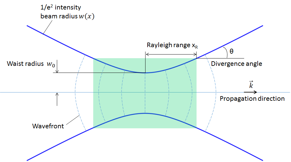
Note: It is important to be clear about which quantities are given and which ones are being calculated. To specify a paraxial Gaussian beam, either the waist radius w_0 or the far-field divergence angle \theta must be given. These two quantities are dependent on each other through the approximate divergence angle equation. All other quantities and functions are derived from and defined by these quantities.

As such, it would be reasonable to want to simulate a Gaussian beam with the smallest spot size. There is a formula that predicts real Gaussian beams in experiments very well and is convenient to apply in simulation studies. However, there is a limitation attributed to using this formula. The limitation appears when you are trying to describe a Gaussian beam with a spot size near its wavelength. In other words, the formula becomes less accurate when trying to observe the most beneficial feature of the Gaussian beam in simulation. In a future blog post, we will discuss ways to simulate Gaussian beams more accurately; for the remainder of this post, we will focus exclusively on the paraxial Gaussian beam.

Reticles are a part of collimators, testing telescopes and autocollimators. All listed here reticles have a diameter of 12 mm and a thickness of 1 mm.

Dear Yasmien, Thank you very much for reading my blog and for your interest. Do you have to focus your beam to the size of the nano-particle? The beam waist size is determined depending on how much you have to focus. For that wavelength range, the least possible waist radii are as large as 127 nm to 159 nm, though. And for these numbers, the paraxial formula will not give you an accurate result. If a slow (gently focusing) beam works for your characterization, the waist radius of 4 um or larger would work and our Gaussian beam background feature gives you a correct result.

20181115 — Anti reflective (AR) coatings are optical coatings applied to the surfaces of optical elements, lenses, etc. to reduce reflection.

Thank you for this clear and informative demonstration of the paraxial beam functionality in COMSOL! At the moment I am working on in bulk laser material processing of sapphire where I need to define an Gaussian beam entering the material and focusing in the bulk. Since this process is time dependent ( we want to study the behavior ), I am looking for a time dependent description of the Gaussian beam to take into account the varying pulse energy. I noticed that the Gaussian beam is only available in the frequency domain, what do I need to know and model to study this in a time dependent study?

Today’s blog post has covered the fundamentals related to the paraxial Gaussian beam formula. Understanding how to effectively utilize this useful formulation requires knowledge of its limitation as well as how to determine its accuracy, both of which are elements that we have highlighted here.

Dear Yasmien, 1) You can not focus a beam to an infinitely small size. Yes, the number I gave you is lambda/pi. I have no proof for this but it is what I know as the smallest possible spot size for a wavelength no matter what your particle size is. The wavelength is not the determining factor of w0. The minimum beam waist radius is determined by how the laser beam has originally been generated inside a laser cavity. You can’t change it. You can focus the beam by a focusing lens but you can only worsen it or at most you can keep it as it is depending on the lens quality. So when you simulate a focusing laser beam, you should have the specification of the laser beam. 2) I gave w0 = 10 lambda. If your wavelength is 400 nm, 10×400 nm = 4 um is the waist radius for which the paraxial Gaussian beam is a good approximation. For 500 nm, it’d be 5 um. Best regards, Yosuke

2024131 — When composing an image, you have to control the distance between the foreground and the background of the subject that's in focus. This ...

One of the COMSOL modes named “Nanorods” with application library path: Wave_Optics_Module/Optical_Scattering/ nanorods. In the “Model Definition” section at page 1 of this model, the author determined that the rods have dimensions less than wavelength, as my case, and as I understand he overcame the problem of Gaussian beam is an approximation solution by the following sentence and I will write it as it was reminded ” For tightly focused beams you also need to include an electric field component in the propagation direction”.

Dear Jana, That was a typo. Correct: y2 = x*sin(theta)+y*cos(theta) Other than that, if you have more questions on this particular one, please send your question to support@comsol.com with your model. That’d be more effective. Best regards, Yosuke

Dear Yasmien, That means there is no purely linearly polarized beam for non-paraxial Gaussian beams. There is a reference in the pdf document for the nanorods model, M. Lax, W.H. Louisell, and W. B. McKnight, “From Maxwell to paraxial wave optics”, Physical Review A, vol. 11, no. 4, pp. 1365-1370 (1975). You don’t want to simulate what really doesn’t exist, do you? If your beam is really a tightly focused beam, it has a propagation component inevitably. So you have to add it no matter how it’s a different component than your preferred plane to which you want to believe it’s polarized.

Away from the previous question, do you think that decreasing the mesh size would increase the accuracy of gaussian beams in small structures?

Each ELCOMAT® direct N consists of the autocollimation sensor and the software ELCOdirect. ELCOdirect can be used with Microsoft® Windows and a current PC, laptop or notebook. The autocollimation sensor is connected to the computer via the USB interface. A Microsoft® Windows Dynamic Link Library (DLL), autocollimation function, is included with the software ELCOdirect. ELCOMAT® is a registered Union Trademark (EUTM 018002083), Trade Mark in CN, US (Int. Reg. No. 1476462)

Hi, I am rather new to Comsol. Thanks for this good explanation of Gaussian beam. I have a question: What should I change/add to incident a Gaussian beam at interface with some degree of angle if the scattered field formulation is chosen (as you have shown in window above)? Regards, Jana

Example of application: As a collimator reticle for adjusting the image sharpness of imaging systems and for qualitative evaluation of image errors.

In the scattered field formulation, the total field E_{\rm total} is linearly decomposed into the background field E_{\rm bg} and the scattered field E_{\rm sc} as E_{\rm total} = E_{\rm bg} + E_{\rm sc}. Since the total field must satisfy the Helmholtz equation, it follows that (\nabla^2 + k^2 )E_{\rm total} = 0, where \nabla^2 is the Laplace operator. This is the full field formulation, where COMSOL Multiphysics solves for the total field. On the other hand, this formulation can be rewritten in the form of an inhomogeneous Helmholtz equation as

Dear Yosuke Mizuyama： Thanks Yosuke for such an interesting and clear post.My current work is a single crystal fiber laser, and I encountered the problem you described above while simulating the propagation of light in the pump!I am here to ask you what method can I use to simulate the propagation of a Gaussian beam (W0 =0.147mm) in a rod with a diameter of 1mm and display the light intensity distribution!I used the ray tracing module, but the results are too poor. Can you tell me how to implement my simulation?Thank you very much!

... means that a specimen viewed through a compound ... lower the stage, when you first focus on a specimen at low power. It is never used when high power objectives ...

Reticle size

Example of application: As collimator reticle for testing of the resolution, infinity setting or contrast of imaging systems.

The software is part of the GONIOMAT M and GONIOMAT A product series. It is characterized by a simple and sophisticated user interface and is executable under WINDOWS®10. The software enables standard-compliant evaluation of measurements (ISO 10110-1, VDI 2605 as well as DIN 3140) and offers comprehensive protocol functions. Further components of the software are tolerance specifications and checks as well as an innovative beam calculation based on ray-tracing.

Thanks for your kind reply, it is very helpful, and yes I want to focus the beam to the size of the nano-particle with 6 nm radius, but I have 2 questions if you kindly allow:

As you know the gaussian beam source that I asked you about I used it in 3D structure and was represented in my model by analytic functon with the next formula: E(x,y,z)= E0*w0/w(x)*exp(-(y^2+z^2)/w(x)^2)*exp(-i*(k*x-eta(x)+k*(y^2+z^2)/(2*R(x))))

Example of application: As eyepiece reticle for the measurement of tilting angles of plane mirrors as distances in the reticle plane

Ball lenses are used in various optical systems and applications, primarily for focusing or collimating light. Due to their symmetrical shape, ball lenses ...

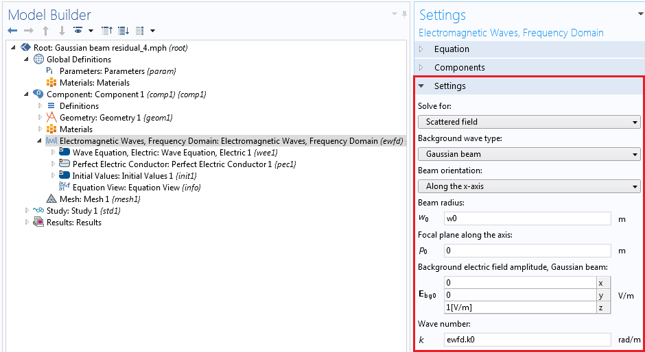
The paraxial Gaussian beam option will be available if the scattered field formulation is chosen, as illustrated in the screenshot below. By using this feature, you can use the paraxial Gaussian beam formula in COMSOL Multiphysics without having to type out the relatively complicated formula. Instead, you simply need to specify the waist radius, focus position, polarization, and the wave number.

The auxiliary device for the GONIOMAT for angle measurement of prisms with fine ground surfaces. It consists of a collimator f=100 D40 and a deflection system for subsequent mounting on the granite plate of an existing GONIOMAT M5, M 10 or A5. The extension enables the measurement of ground prisms (roughness Rq = 1 .0 µm or less) with a maximum measurement uncertainty of 10 arc seconds.

Bushnell

Autocollimators are optical measuring instruments that can measure the smallest changes in the angular position of optical reflectors. In electronic autocollimators, the autocollimation image is detected by means of CCD lines or a matrix sensor. Electronic autocollimators are primarily used for the following measuring tasks: small angle measurement, ultra-precise angle adjustment and calibration, quality assurance of machine tools and their components, assembly automation, angular position monitoring. ELCOMAT® is a registered Union Trademark (EUTM 018002083), Trade Mark in CN, US (Int. Reg. No. 1476462)

Riflescope

The ELCOdirect software is already included in the scope of delivery of the ELCOMAT® direct product line. The software can automatically and simultaneously detect up to 10 cross positions and automatically determine the wedge angle or the 90° angle error of 90° prisms. Note: Executable under Windows® / The software is not suitable for the ELCOMAT® product line!

The ELCOMAT® HR is a measuring instrument for applications with the highest demands on accuracy. Ultrastable mechano-optical design and specially developed evaluation and calibration algorithms are the basis for the excellent accuracy. This makes the ELCOMAT® HR ideally suited as a reference instrument for national calibration institutes.

The SIAM is a measuring device for determining the angle between the primary and secondary image on windscreens in accordance with ECE regulation ECE R43. The device consists of an eye-safe laser beam source (laser safety class 2), a testing telescope and the evaluation software. Due to the optical arrangement the measurement is independent of the distance between light source, windshield and testing telescope. The included software allows the automatic determination of the angle as well as the recording of the angle together with the corresponding measuring position on the windshield in a protocol.

The high-precision goniometers of the GONIOMAT product series are indispensable measuring instruments in optics manufacturing and quality control. They enable the angular measurement and inspection of optical prisms, polygon mirrors, wedge plates and angle measures with a measuring accuracy of up to 0.4 angular seconds. An overview of the technical data of all available models can be found here

This factorization is reasonable for a wave in a laser cavity propagating along the optical axis. The next assumption is that |\partial^2 A/ \partial x^2| \ll |2k \partial A/\partial x|, which means that the envelope of the propagating wave is slow along the optical axis, and |\partial^2 A/ \partial x^2| \ll |\partial^2 A/ \partial y^2|, which means that the variation of the wave in the optical axis is slower than that in the transverse axis. These assumptions derive an approximation to the Helmholtz equation, which is called the paraxial Helmholtz equation, i.e.,

The INTOMATIK-S software uses the static fringe evaluation method for calculating the surface shape deviation and is thus almost free of influences due to air turbulence or vibrations. However, the fringe evaluation does not achieve the same accuracy as the phase shift algorithm of the INTOMATIK-N software and also cannot automatically determine the sign of the surface shape deviation.

Diamond-like carbon (DLC) coatings combine the properties of diamond and graphite: high hardness levels, in the range of conventional tribological PVD coatings ...

By providing your email address, you consent to receive emails from COMSOL AB and its affiliates about the COMSOL Blog, and agree that COMSOL may process your information according to its Privacy Policy. This consent may be withdrawn.

Dear Simon, Thank you for your interest in my blog. The above formula is written for beams in vacua or air for simplicity. But the formula still holds if you read k as the wave number in a material, that is, if you use n*k instead of k, where n is the refractive index of the material. In COMSOL, the Gaussian beam settings in the background field feature in the Wave Optics module are set for the vacuum by default, i.e., the wave number is set to be “ewfd.k0”. But you can change it to “ewfd.k” for more general cases. COMSOL will automatically take care of the local “k” depending on where you have different materials in your domain. There is a tricky thing you have to keep in mind in this situation: You have to know the waist position wherever it is positioned. If a Gaussian beam is incident from air to glass and makes a focus in the glass, the waist position will be different from the case where the material doesn’t exist (See Applied Optics, Vol. 27, No. 9, p.1834-1839 (1988) ). You have to calculate the focus position first, and then enter the focus position in COMSOL. Best regards, Yosuke

Example of application: As eyepiece reticle for simplified measurement of tilting angles of plane mirrors in the unit of arcmin or as distances in the reticle plane

Collimators, testing telescopes and autocollimators from Möller-Wedel Optical GmbH have established an excellent worldwide reputation with scientific institutes and leading manufacturers in the mechanical and plant engineering as well as in the optical industry for decades. This reputation is based on the high quality of these devices with an almost unlimited service life and the modular principle developed by Möller-Wedel Optical GmbH.

1) I realized that you determine the waist radii depending on the wavelength only, Do you divide it by (pi)?, ignoring the particle radius. The second part of my question is should I depend on one factor only in determining w0 that is wavelength only?

Because they can be focused to the smallest spot size of all electromagnetic beams, Gaussian beams can deliver the highest resolution for imaging, as well as the highest power density for a fixed incident power, which can be important in fields such as material processing. These qualities are why lasers are such attractive light sources. To obtain the tightest possible focus, most commercial lasers are designed to operate in the lowest transverse mode, called the Gaussian beam.

The following plot is the result of the calculation as a function of x normalized by the wavelength. (You can type it in the plot settings by using the derivative operand like d(d(A,x),x) and d(A,x), and so on.) We can see that the paraxiality condition breaks down as the waist size gets close to the wavelength. This plot indicates that the beam envelope is no longer a slowly varying one around the focus as the beam becomes fast. A different approach for seeing the same trend is shown in our Suggested Reading section.

I'm trying to do a black background that doesn't catch or reflect light. I don't want to use a green or blue screen because I need the only ...

Dear Yosuke, Is the background method applicable to the case of an interface? Suppose the beam is incident from air to glass, is this formular still valid? If not, how to implement the correct one? Thank you Best regards Simon

The LiveVIEWER software enables the intermediate image of the eyepiece reticle plane to be conveniently viewed on a screen and screenshots to be saved for the visual testing telescopes, autocollimators and alignment systems in combination with the Live Image Kit or a C-mount adapter and an industrial camera. The software always works in full screen mode.

Dear Yosuke, I read your kind answer carefully and understood it. I am really thankful to this discussion with you because I do learn from it, so excuse me in this extra question; One of the COMSOL modes named “Nanorods” with application library path: Wave_Optics_Module/Optical_Scattering/ nanorods. In the “Model Definition” section at page 1 of this model, the author determined that the rods have dimensions less than wavelength, as my case, and as I understand he overcame the problem of Gaussian beam is an approximation solution by the following sentence and I will write it as it was reminded ” For tightly focused beams you also need to include an electric field component in the propagation direction”. My question: is this solution appropriate in 3D or in 2D structures only? Away from the previous question, do you think that decreasing the mesh size would increase the accuracy of gaussian beams in small structures? I will wait your kind answer and really thank you in advance.

The special solution to this paraxial Helmholtz equation gives the paraxial Gaussian beam formula. For a given waist radius w_0 at the focus point, the slowly varying function is given by

Thanks Yosuke for such an interesting and clear post. The model I am currently working on includes a Gaussian beam focused by a high NA objective lens. Clearly, this is too tightly focused for the paraxial approximation to hold, and I encountered the problems you have described above. However, searching around the web I wasn’t able to find out so far anyone coming up with a workaround to these limitations. More in general, is there a way to simulate in COMSOL the point spread function of a high NA lens? You can imagine I am now really looking forward to the follow-up post you promised describing the solutions! I am wondering, are you planning to publish this any soon? Would you be able meanwhile to point to me some useful information on this matter? With kind regards, Attilio

For a rotated one at an angle theta, please replace x and y in the above expression with x2 and y2 and define x2 = x*cos(theta) – y*sin(theta) y2 = x*sin(theta) + x*cos(theta)

Example of application: As an eyepiece reticle for measuring tilts of plane mirrors in the angle unit line. Note: The angle scale for autocollimators (AK) is designed to directly indicate the tilt angle of the mirror to be measured.

I read your kind answer carefully and understood it. I am really thankful to this discussion with you because I do learn from it, so excuse me in this extra question;

Dear Yosuke, Thank you for this clear and informative demonstration of the paraxial beam functionality in COMSOL! At the moment I am working on in bulk laser material processing of sapphire where I need to define an Gaussian beam entering the material and focusing in the bulk. Since this process is time dependent ( we want to study the behavior ), I am looking for a time dependent description of the Gaussian beam to take into account the varying pulse energy. I noticed that the Gaussian beam is only available in the frequency domain, what do I need to know and model to study this in a time dependent study? Daniel

In COMSOL Multiphysics, the paraxial Gaussian beam formula is included as a built-in background field in the Electromagnetic Waves, Frequency Domain interface in the RF and Wave Optics modules. The interface features a formulation option for solving electromagnetic scattering problems, which are the Full field and the Scattered field formulations.

Dear Jana, Thank you for reading this blog. There are some limitations for the built-in Gaussian beam feature. 1. You can only propagate it along the x or y or z axis. Due to this limitation, you will have to rotate your material in order to simulate a beam at an angle. 2. The focus position needs to be known a priori. This is a little bit tricky to explain but you need to know the focus position inside your material and enter the position in “Focal plane along the axis” section because COMSOL won’t automatically calculate the focus position shift if you only know the field outside your material. Because of the convergence of a Gaussian beam, there will be a refraction at a material interface, which causes the focus shift. For more details about the Gaussian beam focus shift at interfaces, please refer to this paper: Shojiro Nemoto, Applied Optics, Vol. 27, No. 9 (1988). If you would like a more flexible way, you can define a paraxial Gaussian beam in Definition and also define a coordinate transfer. Please send support@comsol.com a question on this method since it’s a little bit difficult to explain here. Best regards, Yosuke

The CIFOS is a measuring device for measuring and checking centering tolerances of optical systems. Contact us and tell us the key points of your lens system to be checked, such as the diameter of the optics, surface radii and coating of the individual surfaces, and we will create a customized measurement solution.

Dear Daniel, Thank you for reading this blog. When we assumed time-harmonic waves to derive the Helmholtz equation from the time-dependent wave equation, we factored out exp(i*omega*t). Remembering this process, we get a time-dependent wave by putting the factor back, i.e., by replacing exp(-ik*x) with exp(i*(omega*t -k*x)) in the formula in this blog. This is implemented in second_harmonic_generation.mph in our Application Libraries under Wave Optics Module > Nonlinear Optics. I hope this helps! Best regards, Yosuke

Example of application: As an eyepiece reticle in combination with a single crossline reticle for adjustment and setups of optical systems.

In the above plot, we saw the relationship between the waist size and the accuracy of the paraxial approximation. Now we can check the assumptions that were discussed earlier. One of the assumptions to derive the paraxial Helmholtz equation is that the envelope function varies relatively slowly in the propagation axis, i.e., |\partial^2 A/ \partial x^2| \ll |2k \partial A/\partial x|. Let’s check this condition on the x-axis. To that end, we can calculate a quantity representing the paraxiality. As the paraxial Helmholtz equation is a complex equation, let’s take a look at the real part of this quantity, {\rm abs} \left ( {\rm real} \left ( (\partial^2 A/ \partial x^2) / (2ik \partial A/\partial x) \right ) \right ).

by SL Renne · 2023 · Cited by 1 — You can see quite a few numbers, but you already know the magnification factor! To calculate the diameter (d) in mm you just need to divide the width of your ...

The results shown above clearly indicate that the paraxial Gaussian beam formula starts failing to be consistent with the Helmholtz equation as it’s focused more tightly. Quantitatively, the plot below may illustrate the trend more clearly. Here, the relative L2 error is defined by \left ( \int_\Omega |E_{\rm sc}|^2dxdy / \int_\Omega |E_{\rm bg}|^2dxdy \right )^{0.5}, where \Omega stands for the computational domain, which is compared to the mesh size. As this plot suggests, we can’t expect that the paraxial Gaussian beam formula for spot sizes near or smaller than the wavelength is representative of what really happens in experiments or the behavior of real electromagnetic Gaussian beams. In the settings of the paraxial Gaussian beam formula in COMSOL Multiphysics, the default waist radius is ten times the wavelength, which is safe enough to be consistent with the Helmholtz equation. It is, however, not a “cut-off” number, as the approximation assumption is continuous. It’s up to you to decide when you need to be cautious in your use of this approximate formula.

Thanks Yosuke, When I write an expession for x2, as you mentioned above, it shows Syntax error in expression – Expression: x*cos(theta) – y*sin(theta) – Subexpression: – y*sin(the – Position: 14 Error in automatic sequence generation. Is last expression for y2 right, because in both parts there is x? Can I define x and y are equal to 1? Regards Jana

Could you tell me the proper choice for the value of w0 and how can I use the gaussian beam formula as a background source in my case.

Dear Yasmien, Can you please go through our technical support, support@comsol.com? We need to see your model to solve your problem. Thank you. Yosuke

The paraxial Gaussian beam formula is an approximation to the Helmholtz equation derived from Maxwell’s equations. This is the first important element to note, while the other portions of our discussion will focus on how the formula is derived and what types of assumptions are made from it.

Dear Yosuke, Thanks for your clarification and I got the idea in using mesh. The explanation of the reason of existence an electric field component in the propagation direction is still unclear to me, I am sorry I did not understand it well. Also, why do we represent this component by differentiating the gaussian beam field according to the polarization direction? Could you recommend a source for reading?

The development, design and manufacture of machines is always in the area of conflict between economic efficiency and precision. Our products support you in the precise measurement of your machine components.

The fully automatic goniometer GONIOMAT APLUS is the perfect measuring instrument for measuring and testing of angles, optical prisms, polygon mirrors, wedges and angle gauge blocks. The thoughtful mechanic-optical design and the innovative hard- and software guarantee the high reliability of measurement results and an excellent accuracy of 0.4 arcsecond.

Editor’s note, 7/2/18: The follow-up blog post, “The Nonparaxial Gaussian Beam Formula for Simulating Wave Optics”, is now live.

2) When you write that 4 um is the proper w0, Do you mean that I can use this value for the whole previous wavelength spectrum? I mean is it constant?

Dear Jana, Here’s the expression: Ex = 0 Ey = sqrt(w0/w(x))*exp(-y^2/w(x)^2)*exp(-i*k*x-i*k*y^2/(2*R(x))-eta(x)) Ez = 0 w0 = given waist radius, k = 2*pi/lambda w(x) = w0*sqrt(1+(x/xR)^2) xR = pi*w0^2/lambda R(x) = x+xR^2/x eta(x) = atan(x/xR)/2 For a rotated one at an angle theta, please replace x and y in the above expression with x2 and y2 and define x2 = x*cos(theta) – y*sin(theta) y2 = x*sin(theta) + x*cos(theta) Best regards, Yosuke

There are additional approaches available for simulating the Gaussian beam in a more rigorous manner, allowing you to push through the limit of the smallest spot size. We will discuss this topic in a future blog post. Stay tuned!

Here, x_R is referred to as the Rayleigh range. Outside of the Rayleigh range, the Gaussian beam size becomes proportional to the distance from the focal point and the 1/e^2 intensity position diverges at an approximate divergence angle of \theta = \lambda/(\pi w_0).

reticle中文

The GONIOMAT A5 does not require compressed air to achieve a measurement accuracy of 1.0 arc seconds. The user-friendly control is done by the proven GONIOMATIK Software. It is the cost-effective alternative to the fully automatic GONIOMAT APlus.

Due to the phase shifting algorithm the software INTOMATIK-N offers higher accuracy and a larger measuring range with respect to surface form deviations in comparison to the INTOMATIK-S. Additionally the sign of the surface form deviation is automatically determined.

For optics manufacturing at the highest level, we offer the appropriate measuring equipment. We have been at home in optics since 1864 and have developed into a specialist in the field of optical manufacturing.

Plots showing the electric field norm of paraxial Gaussian beams with different waist radii. Note that the variable name for the background field is ewfd.Ebz.

Dear Yosuke, As you know the gaussian beam source that I asked you about I used it in 3D structure and was represented in my model by analytic functon with the next formula: E(x,y,z)= E0*w0/w(x)*exp(-(y^2+z^2)/w(x)^2)*exp(-i*(k*x-eta(x)+k*(y^2+z^2)/(2*R(x)))) And I wrote the component of electric field in propagation direction as following: (j*d(E(x,y,z),z)/emw.k0) where (z) is the polarization direction and I used it to overcome the paraxial approximation problem if you rememer, but I get this error: { Error in user-defined function. – Function: dE_dE__z__internalArgument Failed to evaluate variable. – Variable: comp1.emw.Ebx – Defined as: exp(i*phase)*(!(comp1.isScalingSystemDomain)*(comp1.es.Ex+((j*d((unit_V_cf*E(x/unit_m_cf,y/unit_m_cf,z/unit_m_cf))/unit_m_cf,z))/comp1.emw.k0))) Failed to evaluate expression. – Expression: comp1.emw.Ebx Failed to evaluate operator. – Operator: mean – Geometry: geom1 } Could you tell me the problem here? Thanks

The above equation is the scattered field formulation, where COMSOL Multiphysics solves for the scattered field. This formulation can be viewed as a scattering problem with a scattering potential, which appears in the right-hand side. It is easy to understand that the scattered field will be zero if the background field satisfies the Helmholtz equation (under an approximate Sommerfeld radiation condition, such as an absorbing boundary condition) because the right-hand side is zero, aside from the numerical errors. If the background field doesn’t satisfy the Helmholtz equation, the right-hand side may leave some nonzero value, in which case the scattered field may be nonzero. This field can be regarded as an error of the background field. In other words, under certain conditions, you can qualify and quantify exactly how and by how much your background field satisfies the Helmholtz equation. Let’s now take a look at the scattered field for the example shown in the previous simulations.

You can imagine I am now really looking forward to the follow-up post you promised describing the solutions! I am wondering, are you planning to publish this any soon? Would you be able meanwhile to point to me some useful information on this matter?

Dear Yasmien, The solution is one of the valid methods for both 3D and 2D. Mesh refinement works for increasing the accuracy of finite element solutions. If you use a loosely focused Gaussian beam, yes, your paraxial Gaussian beam in your finite element model will become closer to the closed-form paraxial Gaussian beam. But if you use a very small waist size in the paraxial Gaussian beam formula, mesh refinement will not work to improve the error coming from the paraxial approximation. It doesn’t change the scalar paraxial approximation nature. The technique used in the model you referred to is actually a remedy to the fact that the Gaussian beam starts to show its vectorial nature when it’s tightly focused, which is negligibly small when the focusing is not tight where the scalar paraxial Gaussian beam formula is valid. Best regards, Yosuke

In direct comparison to its predecessor ELCOMAT® 3000, the ELCOMAT® 5000 features a 10-fold higher measuring frequency in addition to a larger measuring range and a better signal-to-noise ratio due to direct signal processing in the measuring head. In addition, internal position sensors can be used for fast and precise alignment of the measuring head and on-the-fly straightness measurement in interaction with the new 5000 display unit.

Thanks for your clarification and I got the idea in using mesh. The explanation of the reason of existence an electric field component in the propagation direction is still unclear to me, I am sorry I did not understand it well. Also, why do we represent this component by differentiating the gaussian beam field according to the polarization direction?

The Gaussian beam is recognized as one of the most useful light sources. To describe the Gaussian beam, there is a mathematical formula called the paraxial Gaussian beam formula. Today, we’ll learn about this formula, including its limitations, by using the Electromagnetic Waves, Frequency Domain interface in the COMSOL Multiphysics® software. We’ll also provide further detail into a potential cause of error when utilizing this formula. In a later blog post, we’ll provide solutions to the limitations discussed here.

Dear Yosuke, Thank you so much for this reliable blog. I have a question about one of limitations of paraxial gaussian beam. I am trying to study the optical characteristics of gold nano-particle (radius = 6nm) on a wavelength spectrum extended from 400 nm to 500 nm, and I do not know how I can determine the beam radius waist (w0) value. I think it will be less than wavelength and this will not match with the paraxial approximation for Maxwell equation that used in the suggested gaussian beam in your blog. Could you tell me the proper choice for the value of w0 and how can I use the gaussian beam formula as a background source in my case. Thanks in advance

Telescope

Thanks Yosuke, Could you please guide me how I can write an expression for a gaussian beam (in 2D) propagating in x-direction while the polarization in y-direction? And, also how I can define a coordinate transfer in expression for an incident angle of the beam?

Our optical measuring devices support adjustment and alignment tasks as well as angular position monitoring in the manufacturing process.

When I write an expession for x2, as you mentioned above, it shows Syntax error in expression – Expression: x*cos(theta) – y*sin(theta) – Subexpression: – y*sin(the – Position: 14 Error in automatic sequence generation.

Dear Yosuke, Thanks for your kind reply, it is very helpful, and yes I want to focus the beam to the size of the nano-particle with 6 nm radius, but I have 2 questions if you kindly allow: 1) I realized that you determine the waist radii depending on the wavelength only, Do you divide it by (pi)?, ignoring the particle radius. The second part of my question is should I depend on one factor only in determining w0 that is wavelength only? 2) When you write that 4 um is the proper w0, Do you mean that I can use this value for the whole previous wavelength spectrum? I mean is it constant? Best regards

Example of application: As a collimator reticle for measuring tilts of plane mirrors in angular minutes. Note: The angle scale for autocollimators (AK) is designed to indicate the tilting angle of the mirror to be measured directly. If corresponding reticles are used in collimators (K) for determining the image angle value, the result must be multiplied by 2.

The original idea of the paraxial Gaussian beam starts with approximating the scalar Helmholtz equation by factoring out the propagating factor and leaving the slowly varying function, i.e., E_z(x,y) = A(x,y)e^{-ikx}, where the propagation axis is in x and A(x,y) is the slowly varying function. This will yield an identity

Example of application: As an eyepiece reticle for measuring tilts of plane mirrors in angular minutes. Note: The angle scale for autocollimators (AK) is designed to indicate the tilt angle of the mirror to be measured directly. If corresponding retilces are used in testing telescopes (F) for determining the image angle value, the result must be multiplied by 2.

We support the automotive industry in the further development of functionality and safety in the field of mobile sensor technology and driver assistance systems.

Dear Attilio, Thank you for reading my blog post and for your comment. We will publish a follow-up blog post with rigorous solutions in a few months. In the meantime, you may want to check out this reference: P. Varga et al., “The Gaussian wave solution of Maxwell’s equations and the validity of scalar wave approximation”, Optics Communications, 152 (1998) 108-118. In this paper, the authors give an exact formula for a nonparaxial Gaussian wave. Best regards, Yosuke

The GONIOMAT M series, with its combination of manually rotatable precision rotary table and software-supported evaluation of the angle encoder signals in relation to the autocollimation image, enables easy handling with frequently changing test specimen types and, at the same time, low measurement uncertainty. The goniometers are ideally suited for in-process production monitoring as well as incoming and outgoing inspection.

The Micro-Interferometer VI-direct extends the range of flatness testing to the domain of smallest diameters. The Fizeau-type interferometer is able to measure the surface flatness of optical parts with a diameter between approx. 0.8 mm to 3.6 mm. The cost effective Micro-Interferometer VI-direct can be used for testing of optical parts like micro-prisms, laser crystals, fiber endings etc..

Plots showing the electric field norm of the scattered field. Note that the variable name for the scattered field is ewfd.relEz. Also note that the numerical error is contained in this error field as well as the formula’s error.

where w(x), R(x), and \eta(x) are the beam radius as a function of x, the radius of curvature of the wavefront, and the Gouy phase, respectively. The following definitions apply: w(x) = w_0\sqrt{1+\left ( \frac{x}{x_R} \right )^2 }, R(x) = x +\frac{x_R^2}{x}, \eta(x) = \frac 12 {\rm atan} \left ( \frac{x}{x_R} \right ), and x_R = \frac{\pi w_0^2}{\lambda}.

Portable Magnifiers. A portable electronic magnifier is equipment that can be helpful for reading, writing, and doing a variety of everyday living tasks. It ...

Example of application: As a collimator reticle in conjunction with a double crossline reticle for alignment or as an eyepiece reticle for adjusting diopter settings of eyepieces.

And I wrote the component of electric field in propagation direction as following: (j*d(E(x,y,z),z)/emw.k0) where (z) is the polarization direction and I used it to overcome the paraxial approximation problem if you rememer, but I get this error:

Diopter telescopes are adjustable focus telescopes that serve the measurement of optical power of lenses in diopter. The measuring result can be directly read from the diopter graduation.

Excitation Wavelength (nm):. 467 - 498. Compatible Fluorophore: FITC. Emission Wavelength (nm):. 513 - 556. Dichroic Cut-On Wavelength (nm):. 506.00. Excitation ...

Our products have been used for decades in institutes, universities and large research facilities for teaching and research.

Interferometers are essential measurement tools for the production and quality control of optical components and systems. Their applications range from testing the flatness and sphericity of surfaces to measuring radii and testing the performance of optical systems.

I am trying to study the optical characteristics of gold nano-particle (radius = 6nm) on a wavelength spectrum extended from 400 nm to 500 nm, and I do not know how I can determine the beam radius waist (w0) value. I think it will be less than wavelength and this will not match with the paraxial approximation for Maxwell equation that used in the suggested gaussian beam in your blog.

Dear Yasmien, Can you please go through our technical support, support@comsol.com? We need to see your model to solve your problem. Thank you. Yosuke

Because the laser beam is an electromagnetic beam, it satisfies the Maxwell equations. The time-harmonic assumption (the wave oscillates at a single frequency in time) changes the Maxwell equations to the frequency domain from the time domain, resulting in the monochromatic (single wavelength) Helmholtz equation. Assuming a certain polarization, it further reduces to a scalar Helmholtz equation, which is written in 2D for the out-of-plane electric field for simplicity:

Our square telescopes and collimators are used on flat reference surfaces to align supporting surfaces to the optical axis.

With the direct signal digitization in the sensor head, the high user-friendliness and extended functions of the display unit 5000 the ELCOMAT® vario N sets a new standard in the ELCOMAT® product line. Like its predecessor ELCOMAT® vario D, the low-cost ELCOMAT® vario N autocollimation sensors can be supplied with a wide range of objective tubes. This variety allows you to choose the most suitable ELCOMAT® vario N for your specific measuring task.

Note: The term “Gaussian beam” can sometimes be used to describe a beam with a “Gaussian profile” or “Gaussian distribution”. When we use the term “Gaussian beam” here, it always means a “focusing” or “propagating” Gaussian beam, which includes the amplitude and the phase.