Our diagnoses are made by slamming photons into tissue, sometimes using quantum properties of lightv. Therefore, understanding a bit of optics can be useful. The width of the field under the microscope is a function of the eyepiece’s width and the objective’s magnification. These data have been under your nose the whole time. Look at the eyepiece (Fig. 1C). There are two numbers: the first, followed by an “X”, indicates the magnification of the lens; the second, after a “/” is the width of your eyepiece in mm. Now look at your 40X objective (Fig. 1D). You can see quite a few numbers, but you already know the magnification factor! To calculate the diameter (d) in mm you just need to divide the width of your eyepiece (in mm) – called field number (fn) – by all the magnification factors. Often the only one present is the magnification of the objective (mo) so: d = fn/movi. For example, for a 22 mm eyepiece and a 40X objective, in the absence of any further magnification, the diameter of the field is 0.55 mm and the surface is therefore 0.238 mm2.

As pathologists we are used to measure stuff. Ruler and scale are necessary even for autopsies. In surgical pathology, size matters more than weight and residents and pathologist’s assistants measure, ruler at hand, fragments, surgical specimens and tumors. Can we use a ruler under the microscope? Sure! Some tasks – such as measuring the tumor size – can be done with precision under the microscope by sliding a transparent ruler together with the slideiv. Okay, but we need to measure fractions of millimeters. What if we had a teeny-tiny ruler on a glass slide to measure the diameter of the field of view? That would be awesome! Good news, they do exist and they are cheap too! Try to put “stage calibration slide micrometer ruler” in your favorite search engine and you will see an image similar to Figure 1A 14. Before you buy it, check whether someone in your department already has it, hidden and forgotten in a drawer. Once you hold the slide in your hand, the game is clear. Put it under the microscope (you will see Fig. 1B), and do what your – pathologically trained – eyes are doomed to do: meaure with precision the size of your HPF. Slide the last tick to the end of the visible field and count the ticks. Let’s say you counted 0.52 mm, now you can plug this value into the formula to compute the area of a circle starting from the diameter (or use the Tab. I) and voilà you have the surface of your microscope HPF (in our example 0.2124 mm2).

Microscope field of view diameterchart

St Edmund's College Features Live on ITV News Anglia. On Wednesday 20 November, St Edmund's College, Cambridge made it to the 6 o'clock tea […] ...

Effects of miscounting mitoses in GIST. Suppose your microscope has a field of view of 0.52 mm, to count 5 mm2 you will need to count 23.5 HPF (black solid lines). This graph illustrates what happens to your mitotic count when you follow the guidelines and approximate with 20 or with 25 HPF (blue and green dashed lines respectively). How much the sloppy resident would be off? (red dashed lines, counting 50 HPF).

ii Which is, by the way, computed with the following formula: given the diameter d the surface of a circle S is:S = d2*π/4.

Microscope field of view diameterformula

Mitoses can signal biological aggressiveness. Most drugs used in oncology inhibit cell proliferation (unfortunately, not only that of the tumor), and therefore it is wise to limit the use of these drugs in patients who might benefit from them. In most cases, chemotherapy – neoadjuvant or adjuvant – is given in high-grade tumors and we see results since many grading systems use mitotic count 1. In the beginning, mitotic count was reported as the total number of mitoses counted over a surface expressed in number of high-power fields (HPF). The problems with mitotic count are multiple and well-established 2-7. Given that mitoses are identified and recognizedi, quite a few variables can ruin your count: among them delayed fixation can reduce mitotic activity, tumor heterogeneity can limit reproducibility, and thicker slices can increase the count. However, the most discussed variable is the surface area evaluated. Digital pathology will at least solve this problem 8-10, but since it is not implemented in most centers, many pathologists still peer with their own eyes HPFs of different surfaces.

The way a variable ND filter works is by rotating the front filter relative to the back filter. As the filters are rotated, the amount of polarized light that ...

Secure .gov websites use HTTPS A lock ( Lock Locked padlock icon ) or https:// means you've safely connected to the .gov website. Share sensitive information only on official, secure websites.

Field of view microscopeformula

Shop stylish sunglasses for UV protection at Roots. Find the perfect pair to shield your eyes in style.

Mitoses are just part of the picture. They are combined with size and site to compute the risk class 22. This is true also for other pathologies: mitoses do notdetermine grading on their own. To understand the impact let’s look at an example. Figure 3 is a Montecarlo simulation of 10,000 GISTs. First, the simulation generated random sites respecting the proportion reported in literature 18; similarly, it generated mitoses; lastly the simulation produced the sizes as a function of mitoses (easy to imagine why) and the sites (with the idea that an esophageal GIST tends to be smaller because symptoms will appear sooner). Now that we have the largest GIST dataset ever built (just good for this example), let’s play with it and compute the risk class – according to Miettinen and Lasota – for each count. As expected, if you approximate there is almost perfect agreement. The punchline is that even in the worst case scenario (counting 50 HPF instead of 23.5 HPF) there is only a 0.2-fold increase in the high risk class whereas the others are under-diagnosed by a factor of 0.1, with a substantial agreement between the two counting strategies (see Fig. 4 caption for more details). Not too bad.

Impact of miscounting mitoses in GIST. Approximations – low and high – have an almost perfect agreement with the right counting strategy (Cohen’s K of 0.980 and 1.00 respectively), whereas the wrong counting strategy had a substantial agreement with it (Cohen’s K = 0.67). The strength of agreement was evaluated according to Landis and Koch 23. Data generated with a Montecarlo simulation based on descriptive statistics of a series of 2560 cases 18.

Compoundmicroscope field of view diameter

Official websites use .gov A .gov website belongs to an official government organization in the United States.

Have you ever seen an astronomical quadrant? It has something in common with your microscope (and calipers). It is the Vernier scale (named after the French mathematician Pierre Vernier). Look at the stage of the microscope, you will see two opposing rulers – on two of the four sides. Look closer (Fig. 1E). The shorter ruler is not perfectly aligned to the longer one, it is fine. This is the Vernier scale. It allows you to measure lengths with the precision of 0.1 mm. How does it work? Align the two 0 on the two rulers, the tenth tick of the shorter ruler will be on the ninth tick of the longer one. The latter is a regular ruler with the ticks in millimeters. The shorter one shows the ticks at 0.9 mm, therefore when the zeros are aligned, the tenth tick falls on the ninth tick of the longer ruler (9 mm). Gently move the stage and the rulers will misalign (Fig. 1F). Now to understand how much you moved, you have to see where the zero of the short ruler falls (this will be the millimeters you moved) and which tick of the short ruler aligns with the tick of the long one (this will be the tenth of mm you moved). Although this method might help you when navigating with an astronomical quadrant, it is the most complicated presented and also the least accurate (only to 0.1 mm).

Grin (26 jan. 1920–17 août 2022), ID de mémorial Find a Grave 255219141, faisant référence à Monterey City Cemetery, Monterey, Monterey County, California, ...

Inconel is a metallic alloy that ensures flat spectral response from the UV to the near IR. Unprotected metal coatings like this should only be cleaned by blown ...

iii For example, in Practical Soft Tissue Pathology 11 – a book that I like and encourage to read – the author reports “5 mm2 is equivalent to approximately 20 high-power (40×) fields” (p. 470); similarly the Cancer Protocol Templates of the College of American Pathologists of GIST states “5 mmq approximated with 20-25 HPF” 12.

Apr 15, 2024 — Calculating Field of View · 1. Determine your imager's Field of View (in degrees) from the manufacturer's specs. · 2. Divide the value from Step ...

Counting stuff under the microscope is part of the duties of a surgical pathologist. Many textbooks and articles still report the surface area as the number of high-power fields (HPFs) counted. This is bad, since the area displayed by an HPF varies between two microscopes. It is therefore necessary to express the surface as mm2. This is a how to guide written for the resident who has to measure the HPF of the microscope for the first time. The Resident can either calibrate the microscope with a stage micrometer slide (a small ruler on a glass slide) or compute the surface area of the HPF using the numbers on the eyepiece and the magnification objective. for “10X/22” eyepiece and a “40X” objective, the diameter of the HPF is 22/40 = 0.55 (if no other magnification is present), and the surface is 0.238 mm2. The young resident might then ask: “How far off-target was I when I counted the number of HPFs that the chief resident declared to be correct?” Probably not that much: although legitimate in principle and correct in math, the size of the problem is often overstated since microscopes are not that different after all and because pathology is not just about counting.

This is an open access journal distributed in accordance with the CC-BY-NC-ND (Creative Commons Attribution-NonCommercial-NoDerivatives 4.0 International) license: the work can be used by mentioning the author and the license, but only for non-commercial purposes and only in the original version. For further information: https://creativecommons.org/licenses/by-nc-nd/4.0/deed.en

Microscope field of view diameterpdf

Now you have the size of your field of view. You might ask: “How far off-target was I?” The terms of the problem were stated by Ellis and Whitehead. In 1981 they surveyed all the microscopes marketed at the time and hypothesized a grim scenario by comparing the performance of the two extreme microscopes resulting in a 6-fold difference 2. This result led them to question the value of mitotic count as a marker of malignancy (in the context of smooth muscle tumor). The paper is often cited as seminal in recognizing the problem of HPF 1, an it is thus useful to give it a look. Gazing at the plotted numbers, they are not so bad. Seventy percent of the marketed microscopes have a median field of view equal to 0.38 mm with an interquartile range (IQR) of 0.35-0.45 mm – note that the upper limit is close to the modern microscopesvii. The remaining 8 marketed microscopes depart from the previous group, with a median field of view of 0.66 mm (IQR 0.6-0.7 mm). They were outliers at the time and would be outliers today as well. Let’s use the data at hand: in their example of 5 mitoses per mm, it is true that the extreme microscopes would give very different counts (4 vs. 21), but if we do a simple summary statistics of the counts instead of comparing the extremes, numbers are not so grim (median is 8 mitoses and IQR 5-14; i.e. half of the counts differ at most by 9 mitoses), and today they would be even less so - with less variation among the marketed microscopes. Moreover, what is most reassuring is that outliers are rare in the market: the bulk of the microscopes out there are alike and therefore the scenario is further tempered.

Graphical representation of the data from the seminal paper of Ellis and Whitehead 2. The overall median and IQR are represented by the solid black line and the gray shade; the median and IQR of the two types of microscopes are in colored dashed lines and shades: this representation clearly shows the outliers (in green).

Field of view microscope40x

Microscope field of view diametertable

Pull over 99.95% of light through the lens to your eyes. Cosmetics: Lenses are very clear with no surface glare. Lenses: Mojo Standard AR. BluBlock AR Coating ...

Correspondence Salvatore Lorenzo Renne Assistant Professor of Pathology, Anatomic Pathology Unit, Humanitas Research Hospital, via Manzoni 56, 20089 Rozzano (MI), Italy E-mail: salvatore.renne@hunimed.eu

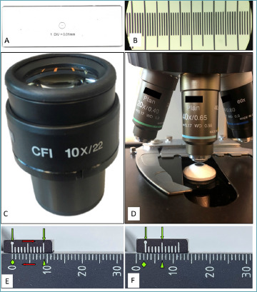
Three ways – two useful – to calculate the diameter of the field of view. The top panels show the stage micrometer slide method: to measure your field of view, bring the thing (A), put it under the microscope and count the ticks (B); in this case each tick is at 0.01 mm of distance. Middle panels show an eyepiece (C) and an objective (D): a simple division will provide you the size of your field of view. Lower panels shows how to use the Vernier scale. The lower ruler shows millimeters, the up- per shows ticks at 0.9 mm. When the zeros are aligned (E, green diamond), the tenth tick of the small ruler falls on nine millimeters (E, arrowhead). Sliding the slides (E, red arrows), the rulers will misalign the zero tick on the small ruler falls after 2 mm (F, green diamond) and the fifth tick of the upper ruler aligns with the lower one, meaning that it moved of 0.5 mm (F, green arrowhead), therefore the two rulers slide for 2.5 mm.

vi In websites describing this procedure 16,17 you will also find reported the tube lens magnification factor that refers to the tube that often connects a fixed camera to the microscope; the point is that any magnification (mx) intervening before the eyepiece shall be counted, and magnifications multiply. Thus, the extended formula is d = fn/(mo*mx).

Microscope field of view diametercalculator

Since we will soon be confronted with machines, it is time to be precise and accurate. To do this with your peers, you need to know the size of your HPF. Now you know how to measure it. Do it now! Lastly, even in the worst case scenario, the results are not so grim, and pathology is not just counting.

May 7, 2013 — Canon MTF charts for EF-S and EF-M lenses — made exclusively for smaller APS-C sensor cameras, such as the EOS Rebel series and EOS M-series — ...

How to consistently assess the same surface area? Most of the Blue Books by the WHO report a table that converts diameter to surface (Tab. I). Useful, if you forgot how to compute the area of a circle starting from the diameterii, but you know the diameter of your field of view with an accuracy of 10 μm. Every medical student or pathology resident approaching the microscope for the first time wrestles with the calculation of field diameter. Some win, and timidly write the numbers with a permanent marker on the microscope base, many others – encouraged by prominent textbooks, popular guidelinesiii and older colleagues – wave their hands and approximate. Here we will review three ways to accomplish this task.

Today, with less variation among marketed microscopes, problems might instead arise when the numbers of HPFs reported in papers and books are naively applied without converting them in mm2. Since the error is multiplicative, the worst case scenario is when you repeat it the most. The mitotic figures in gastrointestinal stromal tumors (GISTs) are counted over 5 mm2, although even recent papers on prominent journals report the surface in 50 HPF 18-21. We read that books and guidelines tell you to approximate 5 mm2 counting between 20 and 25 HPF. If you are not aware of the trick you might also be tempted to count 50 HPF. Now, the bright line in GIST is 5 mitoses/5 mm2: there would be no difference in counts when approximating, whereas using the wrong counting strategy, that uses naively 50 HPF, overestimates the number of mitoses, reporting 5 of them when there were 3 instead (Fig. 2). This may be a problem.

Precision optical pinholes with pinhole aperture diameters from 10 μm to 100 μm. Optical apertures can be used for laser alignment purposes and diffraction ...

Mar 23, 2023 — We can observe single slit diffraction when light passes through a single slit whose width (w) is on the order of the wavelength of the light.

i Basophilic, dark, hairy material (the chromosomes) must be present, either clotted (as in the beginning of metaphase), in a plane (as in metaphase and anaphase), or in separate clots (as in telophase) 6.