0.8x 4

In most cases the material between the objective and sample is air, and “n” equals 1.00. For water, it’s refractive index is 1.33, and specialized immersion oil for microscopy is 1.52. For a low magnification objective such as a 4X or even a 10X, the typical depth of field is plus or minus 3 to 5 microns. In that case, if the sample is very flat, focusing may not be required at all, or only one needs to happen one time. Generally speaking, samples vary in thickness and they vary in flatness, so focusing is required.

Converting from decimals to fractions is straightforward. It does, however, require the understanding that each decimal place to the right of the decimal point represents a power of 10; the first decimal place being 101, the second 102, the third 103, and so on. Simply determine what power of 10 the decimal extends to, use that power of 10 as the denominator, enter each number to the right of the decimal point as the numerator, and simplify. For example, looking at the number 0.1234, the number 4 is in the fourth decimal place, which constitutes 104, or 10,000. This would make the fraction 123410000, which simplifies to 6175000, since the greatest common factor between the numerator and denominator is 2.

In mathematics, a fraction is a number that represents a part of a whole. It consists of a numerator and a denominator. The numerator represents the number of equal parts of a whole, while the denominator is the total number of parts that make up said whole. For example, in the fraction of 38, the numerator is 3, and the denominator is 8. A more illustrative example could involve a pie with 8 slices. 1 of those 8 slices would constitute the numerator of a fraction, while the total of 8 slices that comprises the whole pie would be the denominator. If a person were to eat 3 slices, the remaining fraction of the pie would therefore be 58 as shown in the image to the right. Note that the denominator of a fraction cannot be 0, as it would make the fraction undefined. Fractions can undergo many different operations, some of which are mentioned below.

0.8 x2

When it comes to digital imaging sensors, there is a wide variety to choose from. The main camera sensors used are CCD (charge-coupled device) or CMOS, Complementary Metal Oxide Semiconductor. For cutting edge performance, to reduce read noise, large and expensive cameras exist with liquid or Peltier coolers (deep cooled to about -60 degrees Celsius). Also, EMCCD (Electron Multiplied CCD) cameras allow for single photon detection and are popular for live cell imaging applications. Learn more about key aspects of image sensors common to both CCD and CMOS devices, starting at the pixel level in our "CCD Image Sensors" whitepaper.

For 20X magnification, which can be a numerical aperture of 0.6 to 0.8, the depth of field drops to about plus or minus 500 nanometers. Moving into high magnification with oil immersion at a numerical aperture of 1.47, the depth of field drops very dramatically, And the depth of field could be plus or minus 0.1 to 0.2 microns (100 – 200 nm). That’s a very tight tolerance. At 100 nanometers or 200 nanometers, very tiny changes in flatness of the sample or the height of the sample, or the precision of the guideways of the XY sample motion stage, will make it tricky to stay in focus. For maintaining focus in this situation, a continuous tracking laser auto-focus system connected to a high bandwidth objective focusing stage, such as the DOF-5, is the ideal way to maintain focus in these high numerical aperture, high-resolution applications.

When designing automated digital microscopy devices for life science, biomedical, and diagnostic applications, typically, our goal is to optimize the device for the highest resolution image and the highest throughput in images per second. Microscope calculations such as magnification, resolution, microscope field of view, depth of field, and numerical aperture help us determine various aspects of a microscope’s capabilities and simplify the modeling and prototyping process. In this article, we will cover the importance of microscope calculations in optimizing microscope performance for your specific application.

0.8 x10

The sample is throwing light out in all directions and the job of the objective is to collect as much of that light as possible. The way to do that is to have a high numerical aperture, a big wide cone. If the objective doesn’t collect a wide-angle of the cone, for example, a long working distance, low power objective will merely be getting the light that’s going straight through. That is why numerical aperture is the key to high-resolution imaging. There is one other variable that can be adjusted. By using bluer light, the resolution can be increased, but for a particular application, that may not be possible. Generally speaking, for any given objective, it is worth it to pay to get the highest possible numerical aperture, but there is a slight downside to that.

This process can be used for any number of fractions. Just multiply the numerators and denominators of each fraction in the problem by the product of the denominators of all the other fractions (not including its own respective denominator) in the problem.

In addition to affecting the observation of the specimen itself, the field of view can also impact the ability to capture high-quality images and videos. A larger field of view requires a larger camera sensor or eyepiece, which can increase the cost of the microscope system. It is essential to consider the balance between field of view, magnification, and cost when selecting and optimizing a microscope for a particular application.

A larger field of view is generally desirable, as it allows for a larger area of the sample to be viewed at once, making it easier to locate and navigate to specific areas of interest. However, as the magnification increases, the field of view decreases, making it more difficult to observe larger areas of the specimen at higher magnifications. Need help with microscope calculations? Download our calculator.

0.8 x 125astro tech

The first multiple they all share is 12, so this is the least common multiple. To complete an addition (or subtraction) problem, multiply the numerators and denominators of each fraction in the problem by whatever value will make the denominators 12, then add the numerators.

Microscope calculations are specific to the imaging sensor and microscope objective selection, which also impacts the performance requirements of the sample XY motion and Z focusing motion.

Besides the magnification, reducing the size of the sensor down to the size of the field of view on the sample also does the same with the pixels. For example, a sensor with 4 micron pixels and a 40X objective would be 0.1 micron of geometric resolution or 100 nanometers. But it turns out it isn’t quite that simple. There’s a property of light that acts like a particle, the photon. It also has a wave property. The wave nature of light leads to a condition called diffraction, and due to diffraction, limits are set on resolution. To better understand how that works, we need to explore another concept, which is called numerical aperture.

Similarly, fractions with denominators that are powers of 10 (or can be converted to powers of 10) can be translated to decimal form using the same principles. Take the fraction 12 for example. To convert this fraction into a decimal, first convert it into the fraction of 510. Knowing that the first decimal place represents 10-1, 510 can be converted to 0.5. If the fraction were instead 5100, the decimal would then be 0.05, and so on. Beyond this, converting fractions into decimals requires the operation of long division.

The same thing occurs in traditional photography, a very small aperture will increase the depth of field. A higher numerical aperture will give a higher resolution, but the depth of field becomes considerably smaller. There is a distance above the sample plane and a distance below the sample plane, and anywhere within them, there is essentially perfect focus. As soon as the objective and sample are outside of that boundary, the image begins to blur.

It is often easier to work with simplified fractions. As such, fraction solutions are commonly expressed in their simplified forms. 220440 for example, is more cumbersome than 12. The calculator provided returns fraction inputs in both improper fraction form as well as mixed number form. In both cases, fractions are presented in their lowest forms by dividing both numerator and denominator by their greatest common factor.

The microscope field of view stands for the area of the sample visible through the microscope, which is calculated by dividing the sensor diagonal size by the magnification of the objective lens. For instance, a 20 mm diagonal sensor with a 20X objective lens would yield a Field Of View (FOV) of 1 mm, typical for microscopy applications. Microscope field of view can be calculated using the following formula:

Covers key formulas for selecting the optimal imaging sensor and microscope objective for your digital imaging application including sensor size, magnification, field of view, pixel sizes, resolution, depth of field, and numerical aperture.

where Sensor Diagonal is the diagonal size of the camera sensor in millimeters (similar to specifying a TV size), and Objective Magnification is the magnification of the objective lens being used.

0.8 x120

0.8 x 125calculator

The image below shows a variety of microscope systems. There are multiple magnification objectives depicted: low power 4x, medium power, 40x and high power 100x. The distance from the end of the objective to the sample, which is called the working distance, is going to be larger on a low power objective, less on a medium power and very fine, possibly a fraction of a millimeter for the high power system. What’s critical is the angle. The sample is illuminated and light is coming out of it. In the case of the shorter working distance, higher numerical aperture objectives, that light is coming at an increasingly higher angle. The Numerical Aperture (NA) of the objective equals the sine of the half-angle (theta divided by two where theta is the entire angle). Read more on how to calculate the numerical aperture.

In the previous example we considered a sensor with 4 micron pixels used with an objective with 40X magnification and a numerical aperture of 0.8. The sensor and magnification provide 100 nm geometric resolution. However, due to diffraction, the sample image resolution will be greater than 100 nm. For example, yellow green light has a wavelength lambda of 550 nm. Using the above equation, the diffraction limited resolution is actually 419 nm. Therefore, the resolution of the sample is > 4 times the geometric resolution at the camera sensor which results in oversampling. While some oversampling is appropriate, 4 times is excessive and a waste of sensor pixels. Calculate the diffraction using our calculator.

For a low power 4x system, the numerical aperture is going to be very low, on the order of 0.05 to 0.1. In a medium power 40x system, it could be in the range of 0.5 to 0.8 and for a high power system, it can be as high as 0.9 or 0.95. As long as there is air between the objective and the sample, the numerical aperture can never exceed 1. When imaging slides, in order to exceed an NA of 1, a liquid can be added between the coverslip and the objective. Typically, oil or water are used for this and the objectives are referred to as oil immersion or water immersion objectives. With water, the numerical aperture goes up to about 1.1 and using oil, the numerical aperture can go up to as high as 1.47.

The consequence of numerical aperture is that it directly relates to the Depth Of Field (DOF). For a given objective, looking at a sample, there’s a particular plane of perfect focus. The depth of field is, how far above and below that plane the objective and sample can be and still have everything in focus.

0.8x 3

An alternative method for finding a common denominator is to determine the least common multiple (LCM) for the denominators, then add or subtract the numerators as one would an integer. Using the least common multiple can be more efficient and is more likely to result in a fraction in simplified form. In the example above, the denominators were 4, 6, and 2. The least common multiple is the first shared multiple of these three numbers.

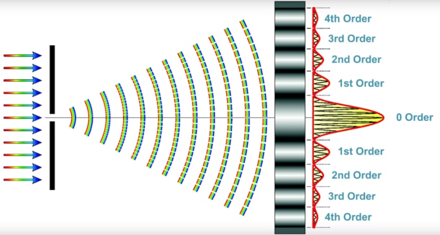
To better understand diffraction imagine if light moved strictly in straight lines. If a pinhole is illuminated with some light, the light would be directed in a straight beam. What actually happens is due to the wave nature of light, the light is diffracted, and instead of going straight, it spreads out into a cone. As shown in the diffraction image, the brightest light is the zero-order straight through, then the intensity decreases for the first order, second order, third order, etc. Unless the objective is capturing all of those higher orders, it is difficult to synthesize a high-resolution image. This describes what the fine structure of your sample is doing, it could be cells, chromosomes, or nuclei, and all of that fine structure spreads the light out.

To optimize the field of view for a particular application, it is vital to consider the size of the specimen and the level of detail required. For example, if a large sample with low detail is being observed, a lower magnification and larger field of view may be more appropriate. Conversely, if a smaller specimen with high detail is being observed, a higher magnification and smaller field of view may be necessary to achieve the desired level of resolution.

0.8 x5

The process for dividing fractions is similar to that for multiplying fractions. In order to divide fractions, the fraction in the numerator is multiplied by the reciprocal of the fraction in the denominator. The reciprocal of a number a is simply 1a. When a is a fraction, this essentially involves exchanging the position of the numerator and the denominator. The reciprocal of the fraction 34 would therefore be 43. Refer to the equations below for clarification.

Fraction subtraction is essentially the same as fraction addition. A common denominator is required for the operation to occur. Refer to the addition section as well as the equations below for clarification.

Multiplying fractions is fairly straightforward. Unlike adding and subtracting, it is not necessary to compute a common denominator in order to multiply fractions. Simply, the numerators and denominators of each fraction are multiplied, and the result forms a new numerator and denominator. If possible, the solution should be simplified. Refer to the equations below for clarification.

Unlike adding and subtracting integers such as 2 and 8, fractions require a common denominator to undergo these operations. One method for finding a common denominator involves multiplying the numerators and denominators of all of the fractions involved by the product of the denominators of each fraction. Multiplying all of the denominators ensures that the new denominator is certain to be a multiple of each individual denominator. The numerators also need to be multiplied by the appropriate factors to preserve the value of the fraction as a whole. This is arguably the simplest way to ensure that the fractions have a common denominator. However, in most cases, the solutions to these equations will not appear in simplified form (the provided calculator computes the simplification automatically). Below is an example using this method.

In this video, we will explain key optical imaging formulas and how they help in designing your automated digital microscopy imaging applications. Download Microscopy Calculator

This is called the depth of field. The formula for the depth of field is: where: “n” is the refractive index of the material between the objective and the sample λ (lambda) is the wavelength of light NA is the Numerical Aperture

To summarize, for high imaging resolution a high numerical aperture objective is required and one of the consequences of that is a fairly small depth of field which places an emphasis on the quality and performance of your focusing stage and XY sample positioning stage. Dover Motion has developed the DOF-5 specifically for microscope objective focusing.

Below are multiple fraction calculators capable of addition, subtraction, multiplication, division, simplification, and conversion between fractions and decimals. Fields above the solid black line represent the numerator, while fields below represent the denominator.