This mini-project consisted of two parts. First, we looked at how the laser beam from a green laser pointer diverges with increasing distance. This part of the experiment was done in the long hallway outside the lab, where we could place the laser as much as several hundred feet away from the screen. Later we measured the intensity profile of a red HeNe laser by a much more precise method at distances that were mostly less than one meter from the laser. Our results showed that the profile is not linear as we originally expected, but rather is curved. The actual hyperbolic shape is approximately constant near the laser and diverges in proportion to distance in the far field, due to diffraction.

Gaussian beamintensity formula

WinLens3D Basic: lens design software. Free version of the WinLens3D optical design package, which provides serious design and analysis tools for optical ...

Many people have the idea that laser beams are perfectly parallel "lines of light." Initially, we also held this naive belief, but Dr. Noe challenged our misunderstanding by demonstrating that the beam from a green laser pointer clearly diverges. But how does the size of the laser beam relate to the distance to the screen? We hypothesized that the beam width could not be directly proportional to the distance because if that were true, extrapolating back to a distance of zero from the laser would produce a beam size of zero, which just didn’t make sense. We believed that the relationship would be linear, but rather than being directly proportional the diameter and distance would be related by an equation of the form ax + b, where a is the rate of divergence and b is the initial diameter at zero distance.

Gaussian beamcalculator

We can determine the length of the laser cavity by finding the beat frequency between the longitudinal modes of the laser. The equation of beat frequency is where c is the speed of light. With help from Vince [link] we found a beat frequency of 685.81 MHz, which corresponds to L = 21.8 cm. This result is in reasonable agreement with our conclusion that the waist is 3.6 cm behind the face of the laser, since the total length of the laser is 27.0 cm. By finding the divergence of the laser beam, which explains how the beam diffracts at large distances as the hyperbolic curve approaches a line, we were able to calculate the wavelength of the laser beam. The beam's divergence, theta, is described by the equation: [4] Equation[4] can be used to find the wavelength of the laser beam by using the approximate slope of the curve as the divergence. Using a divergence of 6.568 radians, and a waist size of 299.3 micrometers, we found that the wavelength of the laser was 617.58 nanometers. The error in this calculation is only 2.28 percent, when compared to the theoretical value of the laser, which was 632 nanometers. Conclusion In this project we learned not only about the changing profile and propagation of a laser beam, we also discovered how to determine the length and mirror configuration of the laser cavity. Finally, we learned that careful measurements of the beam profile such as ours can even be used to roughly determine the wavelength of the laser! References [1] Enrique J. Galvez. "Gaussian beams in the optics course." Am. J. Phys. 74, xxx-xxx (2006).

Our results are shown in Figure 5. We found that the waist position was 3.6 cm behind the front face of the laser, which must therefore be where the surface of the output coupler mirror is. We also found w0 = 299.3 microns, which corresponds to a Rayleigh range [1] of 444 mm.

The razor blade was taped to a right-angle bracket that was attached to a micrometer-driven translation stage. We moved in steps of either 1 or 2 mils. (One mil equals 0.001 inch or 25.4 microns.) We made these measurements at 31 different distances under 70 mm and also at 300 mm. In all, we wrote down and entered over 1000 data points by hand. In retrospect we took more data than we needed. Fewer width measurements over more evenly spaced distances would have been sufficient.

Gaussian beamwaist

Download scientific diagram | The beam quality factor M 2 of a typical laser beam with k = 850 nm and k = 1550 nm versus C 2 n for four values of beam ...

In this project we learned not only about the changing profile and propagation of a laser beam, we also discovered how to determine the length and mirror configuration of the laser cavity. Finally, we learned that careful measurements of the beam profile such as ours can even be used to roughly determine the wavelength of the laser!

Personalize your world with our 3D Crystal Photo Cube! This crystal cube contains a 3D laser-engraved photo, guaranteeing a one-of-a-kind keepsake that will ...

Gaussian Beam Propagation. Note: this calculation is only valid for paraxial rays and where the thickness variation across the lens is negligable.

Gaussian beamdivergence

Gaussian beam laserpdf

In this equation r is the distance from the center of the beam and A(z) and w(z) describes the peak intensity and width of the beam, which both change with distance z along the beam. I(r) can be measured directly by moving a pinhole across the beam and recording how much light passes through it, as this past LTC student did. Unfortunately one needs a very tiny pinhole or narrow slit to get accurate results where the beam is very small. A better method is to gradually cut off the beam by moving a razor blade into it, as shown in this figure.

Gaussian beampdf

The fluorescence emitted by the DNA chip was captured by the imaging lens and the CCD camera, so for a clear fluorescent image it was necessary to ensure high resolution of the imaging system. A 1951 USAF resolution test chart (Figure 13) can be used to measure the resolution level of a camera imaging system. The largest set of short lines on the chart that the imaging system can resolve is its resolution.

The five kinematic equations are a set of formulas used to describe the motion of an object in one dimension, also known as linear motion. Each equation relates ...

The diameter of the field in an optical microscope is expressed by the field-of-view number, or simply the field number, which is the diameter of the view ...

9 PIECE HEX KEY SET ALLEN KEYS ALAN POINT END 1.5mm - 10mm EXTRA LONG NEW 23-81. partsdaddyuk (129867); 99.6% positive feedback. Approx. C $11.61. GBP 6.45.

Our green laser was held on a small tripod stand that sat on the ground, and was pointed at the wall at the end of the hallway. Each of us separately visually estimated the diameter of the laser spot on the wall using a meter stick. We repeated this procedure at several distances from the wall, from 35 meters (116 feet) up to about 141 meters (480 feet). We used a 25 foot tape measure to make marks every 25 feet in the hallway to make measuring the distances more convenient.

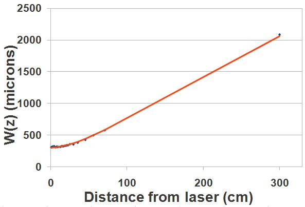
where w0 is the beam width at its minimum value, or "beam waist," zwaist is the distance of the beam waist from the face of the laser, and λ is the wavelength of the laser. A positive zwaist means the waist is in front of the laser's front face. Our results are shown in Figure 5. We found that the waist position was 3.6 cm behind the front face of the laser, which must therefore be where the surface of the output coupler mirror is. We also found w0 = 299.3 microns, which corresponds to a Rayleigh range [1] of 444 mm. Figure 5. Measured and best-fit beam profile. We can determine the length of the laser cavity by finding the beat frequency between the longitudinal modes of the laser. The equation of beat frequency is where c is the speed of light. With help from Vince [link] we found a beat frequency of 685.81 MHz, which corresponds to L = 21.8 cm. This result is in reasonable agreement with our conclusion that the waist is 3.6 cm behind the face of the laser, since the total length of the laser is 27.0 cm. By finding the divergence of the laser beam, which explains how the beam diffracts at large distances as the hyperbolic curve approaches a line, we were able to calculate the wavelength of the laser beam. The beam's divergence, theta, is described by the equation: [4] Equation[4] can be used to find the wavelength of the laser beam by using the approximate slope of the curve as the divergence. Using a divergence of 6.568 radians, and a waist size of 299.3 micrometers, we found that the wavelength of the laser was 617.58 nanometers. The error in this calculation is only 2.28 percent, when compared to the theoretical value of the laser, which was 632 nanometers. Conclusion In this project we learned not only about the changing profile and propagation of a laser beam, we also discovered how to determine the length and mirror configuration of the laser cavity. Finally, we learned that careful measurements of the beam profile such as ours can even be used to roughly determine the wavelength of the laser! References [1] Enrique J. Galvez. "Gaussian beams in the optics course." Am. J. Phys. 74, xxx-xxx (2006).

In this case the changing intensity of the part of the beam that's not cut off is given by an integral like this, where x is the position of the blade. The theoretical curve given by this integral can be matched to the data points by a least-squares method like we used before. The result is the width w of the laser beam at some particular distance from the laser. 2. Setup and Procedure Figure 3 shows our setup. We initially used the same green laser pointer as before but unfortunately the characteristics of its beam suddenly changed when a new battery was used, possibly due to damage to its crystal. Therefore we switched to the very stable red HeNe laser shown. The photodetector was a Thorlabs DET110 whose current was read by a multimeter. We placed a converging lens ahead of the detector to ensure that none of the beam missed the detector. As shown the detector was intentionally placed away from the exact focus of the lens to avoid possibly damaging the detector. Figure 3a. A bird's eye view of the experimental setup Figure 3b. A picture of the setup The razor blade was taped to a right-angle bracket that was attached to a micrometer-driven translation stage. We moved in steps of either 1 or 2 mils. (One mil equals 0.001 inch or 25.4 microns.) We made these measurements at 31 different distances under 70 mm and also at 300 mm. In all, we wrote down and entered over 1000 data points by hand. In retrospect we took more data than we needed. Fewer width measurements over more evenly spaced distances would have been sufficient. 3. Analysis and Results Two types of analysis were done - (a) finding the beam width w(z) at each of the 32 distances and (b) constructing the beam profile from these results. Both used the least-squares method that was employed previously with the green laser pointer data. When finding the beam width by the least squares method one has the problem that the theoretical function (integral of a Gaussian) can not be written as a formula and thus cannot be directly compared to the data. The integral in fact defines a special function called the "error function," or erf(x). We dealt with this by numerically integrating the trial Gaussian functions and comparing these numerical integral curves to the data. The numerical integral is computed by simply summing all the Gaussian values up to some particular point x. The result of one such least squares analysis is shown in Figure 4. Figure 4. One of 32 sets of width data with its best-fit erf curve. When we plotted the 32 different beam width values, w(z), we found that the points formed a hyperbola. According to the reference below and others, the formula for the hyperbola is where w0 is the beam width at its minimum value, or "beam waist," zwaist is the distance of the beam waist from the face of the laser, and λ is the wavelength of the laser. A positive zwaist means the waist is in front of the laser's front face. Our results are shown in Figure 5. We found that the waist position was 3.6 cm behind the front face of the laser, which must therefore be where the surface of the output coupler mirror is. We also found w0 = 299.3 microns, which corresponds to a Rayleigh range [1] of 444 mm. Figure 5. Measured and best-fit beam profile. We can determine the length of the laser cavity by finding the beat frequency between the longitudinal modes of the laser. The equation of beat frequency is where c is the speed of light. With help from Vince [link] we found a beat frequency of 685.81 MHz, which corresponds to L = 21.8 cm. This result is in reasonable agreement with our conclusion that the waist is 3.6 cm behind the face of the laser, since the total length of the laser is 27.0 cm. By finding the divergence of the laser beam, which explains how the beam diffracts at large distances as the hyperbolic curve approaches a line, we were able to calculate the wavelength of the laser beam. The beam's divergence, theta, is described by the equation: [4] Equation[4] can be used to find the wavelength of the laser beam by using the approximate slope of the curve as the divergence. Using a divergence of 6.568 radians, and a waist size of 299.3 micrometers, we found that the wavelength of the laser was 617.58 nanometers. The error in this calculation is only 2.28 percent, when compared to the theoretical value of the laser, which was 632 nanometers. Conclusion In this project we learned not only about the changing profile and propagation of a laser beam, we also discovered how to determine the length and mirror configuration of the laser cavity. Finally, we learned that careful measurements of the beam profile such as ours can even be used to roughly determine the wavelength of the laser! References [1] Enrique J. Galvez. "Gaussian beams in the optics course." Am. J. Phys. 74, xxx-xxx (2006).

Gaussian beamradius

where c is the speed of light. With help from Vince [link] we found a beat frequency of 685.81 MHz, which corresponds to L = 21.8 cm. This result is in reasonable agreement with our conclusion that the waist is 3.6 cm behind the face of the laser, since the total length of the laser is 27.0 cm. By finding the divergence of the laser beam, which explains how the beam diffracts at large distances as the hyperbolic curve approaches a line, we were able to calculate the wavelength of the laser beam. The beam's divergence, theta, is described by the equation: [4] Equation[4] can be used to find the wavelength of the laser beam by using the approximate slope of the curve as the divergence. Using a divergence of 6.568 radians, and a waist size of 299.3 micrometers, we found that the wavelength of the laser was 617.58 nanometers. The error in this calculation is only 2.28 percent, when compared to the theoretical value of the laser, which was 632 nanometers. Conclusion In this project we learned not only about the changing profile and propagation of a laser beam, we also discovered how to determine the length and mirror configuration of the laser cavity. Finally, we learned that careful measurements of the beam profile such as ours can even be used to roughly determine the wavelength of the laser! References [1] Enrique J. Galvez. "Gaussian beams in the optics course." Am. J. Phys. 74, xxx-xxx (2006).

When we plotted the 32 different beam width values, w(z), we found that the points formed a hyperbola. According to the reference below and others, the formula for the hyperbola is where w0 is the beam width at its minimum value, or "beam waist," zwaist is the distance of the beam waist from the face of the laser, and λ is the wavelength of the laser. A positive zwaist means the waist is in front of the laser's front face. Our results are shown in Figure 5. We found that the waist position was 3.6 cm behind the front face of the laser, which must therefore be where the surface of the output coupler mirror is. We also found w0 = 299.3 microns, which corresponds to a Rayleigh range [1] of 444 mm. Figure 5. Measured and best-fit beam profile. We can determine the length of the laser cavity by finding the beat frequency between the longitudinal modes of the laser. The equation of beat frequency is where c is the speed of light. With help from Vince [link] we found a beat frequency of 685.81 MHz, which corresponds to L = 21.8 cm. This result is in reasonable agreement with our conclusion that the waist is 3.6 cm behind the face of the laser, since the total length of the laser is 27.0 cm. By finding the divergence of the laser beam, which explains how the beam diffracts at large distances as the hyperbolic curve approaches a line, we were able to calculate the wavelength of the laser beam. The beam's divergence, theta, is described by the equation: [4] Equation[4] can be used to find the wavelength of the laser beam by using the approximate slope of the curve as the divergence. Using a divergence of 6.568 radians, and a waist size of 299.3 micrometers, we found that the wavelength of the laser was 617.58 nanometers. The error in this calculation is only 2.28 percent, when compared to the theoretical value of the laser, which was 632 nanometers. Conclusion In this project we learned not only about the changing profile and propagation of a laser beam, we also discovered how to determine the length and mirror configuration of the laser cavity. Finally, we learned that careful measurements of the beam profile such as ours can even be used to roughly determine the wavelength of the laser! References [1] Enrique J. Galvez. "Gaussian beams in the optics course." Am. J. Phys. 74, xxx-xxx (2006).

And is it true that if a power adaptor rated at 12v 600ma can be used as 6v 300ma or 3v 150ma or 1.5volt 75ma? All related (37).

... Angle Night Vision Back Up Camera. +. Backup camera RCA Video Cable,Car Reverse Rear View Parking Camera Video Audio Extension Cable. +. Reversing Backup Camera ...

Figure 3 shows our setup. We initially used the same green laser pointer as before but unfortunately the characteristics of its beam suddenly changed when a new battery was used, possibly due to damage to its crystal. Therefore we switched to the very stable red HeNe laser shown. The photodetector was a Thorlabs DET110 whose current was read by a multimeter. We placed a converging lens ahead of the detector to ensure that none of the beam missed the detector. As shown the detector was intentionally placed away from the exact focus of the lens to avoid possibly damaging the detector.

Two types of analysis were done - (a) finding the beam width w(z) at each of the 32 distances and (b) constructing the beam profile from these results. Both used the least-squares method that was employed previously with the green laser pointer data.

Gaussian beamwaist calculator

Aug 26, 2024 — They impose controls on the supply chain and people are required to justify why they need the higher power devices (as opposed to a lower power ...

When finding the beam width by the least squares method one has the problem that the theoretical function (integral of a Gaussian) can not be written as a formula and thus cannot be directly compared to the data. The integral in fact defines a special function called the "error function," or erf(x). We dealt with this by numerically integrating the trial Gaussian functions and comparing these numerical integral curves to the data. The numerical integral is computed by simply summing all the Gaussian values up to some particular point x. The result of one such least squares analysis is shown in Figure 4. Figure 4. One of 32 sets of width data with its best-fit erf curve. When we plotted the 32 different beam width values, w(z), we found that the points formed a hyperbola. According to the reference below and others, the formula for the hyperbola is where w0 is the beam width at its minimum value, or "beam waist," zwaist is the distance of the beam waist from the face of the laser, and λ is the wavelength of the laser. A positive zwaist means the waist is in front of the laser's front face. Our results are shown in Figure 5. We found that the waist position was 3.6 cm behind the front face of the laser, which must therefore be where the surface of the output coupler mirror is. We also found w0 = 299.3 microns, which corresponds to a Rayleigh range [1] of 444 mm. Figure 5. Measured and best-fit beam profile. We can determine the length of the laser cavity by finding the beat frequency between the longitudinal modes of the laser. The equation of beat frequency is where c is the speed of light. With help from Vince [link] we found a beat frequency of 685.81 MHz, which corresponds to L = 21.8 cm. This result is in reasonable agreement with our conclusion that the waist is 3.6 cm behind the face of the laser, since the total length of the laser is 27.0 cm. By finding the divergence of the laser beam, which explains how the beam diffracts at large distances as the hyperbolic curve approaches a line, we were able to calculate the wavelength of the laser beam. The beam's divergence, theta, is described by the equation: [4] Equation[4] can be used to find the wavelength of the laser beam by using the approximate slope of the curve as the divergence. Using a divergence of 6.568 radians, and a waist size of 299.3 micrometers, we found that the wavelength of the laser was 617.58 nanometers. The error in this calculation is only 2.28 percent, when compared to the theoretical value of the laser, which was 632 nanometers. Conclusion In this project we learned not only about the changing profile and propagation of a laser beam, we also discovered how to determine the length and mirror configuration of the laser cavity. Finally, we learned that careful measurements of the beam profile such as ours can even be used to roughly determine the wavelength of the laser! References [1] Enrique J. Galvez. "Gaussian beams in the optics course." Am. J. Phys. 74, xxx-xxx (2006).

We plotted and analyzed our data in a spreadsheet program. We used the Least Squares Method to determine the slope of the line of form ax + b that best matches the data. This method works by squaring the difference between each corresponding theoretical and experimental value. All of these terms are added together to produce a measure of the total error. By minimizing the total error by changing the parameters, we could find the curve that best represents the data points.

The theoretical curve given by this integral can be matched to the data points by a least-squares method like we used before. The result is the width w of the laser beam at some particular distance from the laser.

If one thinks of an analog signal function as a 1D image (see Figure 17.7), it is rather straightforward to extrapolate to the 2D (and 3D) imaging scenario: the image data now vary in 2D or 3D, but the rest of the imaging and analysis procedures still apply. From the point of view of image resolution, this means that the “bandwidth” of an image must be somehow associated with its “sharpness,” and this is related to the highest spatial frequencies it contains. While in consumer photography, it is often problematic to apply an image analysis along the aforementioned criteria (even an out-of-focus or blurred image may still carry memorable impressions), in scientific imaging and microscopy, access to the proper imaging parameters is in most cases feasible. For example, at the very least, one knows (1) that the diffraction limits the maximum sharpness of the data that can be recorded and (2) that the “spatial frequency response” of a microscope can be defined by a suitable calibration sample [e.g., the “1951 USAF resolution test chart”—see Messina (2006); or the so-called “Siemens Star” target—see Thurman (2011)]. As a consequence of the above considerations, the convention is to adapt the relation between the imaging optics properties (ultimately governed by diffraction limit dAbbé) and the pixel size dpixel of the imaging array detector to obey

The graph above shows our results. It is apparent from the graph that a line passing through the origin (b=0) is sufficient to represent the data. We realized from this initial experiment that we need to measure (profile) the beam diameter much closer to the laser. The beam is very small there so a more exact method is needed.