A region selection window will open. Most of the time you’ll want to select the entire image (or use the same selection as the previous image, if you analyzed an image of the same size). Once you’ve made the selection, a progress bar will appear: reading multiple images goes surprisingly quickly.

For direct data acquisition, use the Device manager to select the device. Open Uniformity Interactive. In the Settings dropdown menu, select Signal averaging, and choose the number of images to average (must be ≥; 128 preferred), and be sure Calculate image^2 while averaging is checked. Then acquire the image.

Image sensor noise is a random variation of pixel levels caused by a number of factors— photons (shot noise), thermal (Johnson noise), dark current noise, and variations in the sensitivity and gain of pixels in the image sensor, sometimes called fixed pattern noise (which we will call spatial nonuniformity here. “Nonuniformity” is preferred in the EMVA standard (§4).

Noise from a real image, shown with increased contrast; 4 display pixels per image pixel. Some 8×8 blocking from (low quality) JPEG processing  is visible.

When this plot is selected in Flatfield (the fixed module), the histogram (available in other plots) is omitted so the entire output can be seen.

GenICam

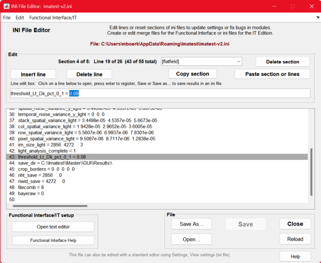
If you have previously run a Flat Field analysis, the [flatfield] section and several ini keys, including threshold_Lt_Dk_pct_0_1 will already exist in the file. Adjust the value of the existing threshold_Lt_Dk_pct_0_1 field in the text editor OR using the INI File Editor tool in the INI dropdown, and save your changes. You can now proceed with analysis as normal.

Strobe lights are the standard for providing visual safety awareness for vehicles, buildings and equipment. Whether you need to provide safety lighting in a building, on equipment or on a vehicle, bright strobing warning lights are a necessity for keeping yourself and your equipment safe. With multiple mounting and power options it is easy to keep your property and employees visible and safely lit with a strong strobe light.

Horizontal and vertical spectrograms and profiles —  described in EMVA §8.3 and 8.4. Combined here. These plots do not contain EMVA required results. Several smoothing settings are available.

From saved image files, select a batch of files, then be sure to select Read n files for pixel-based temporal noise (N >= 4). For EMVA-1288 in the confirmation window.

Introduction  |  EMVA 12288 equations  |  Method  |  Results  |  EMVA & histogram Standard histograms  |  Accumulated histograms  |  H&V spectrograms & profiles | Temporal noise image

Calculating temporal noise and nonuniformity requires that multiple images be captured. (L ≥ 16 is the minimum recommended in EMVA §8; 100-400 is better, but the Imatest calculation will work with as few as 4 images (good for testing-only). The standard recommends capturing a set of light images whose mean pixel level (in linear files with no gamma applied) is 50% of saturation (designated by subscript 50 in the document; we prefer “light”) and also a set of dark pixels (“lens cap on”; designated by subscript dark).

Shipping Policy | Privacy Policy | Return Policy | Imatest Terms and Conditions

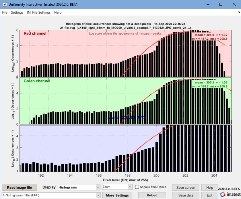
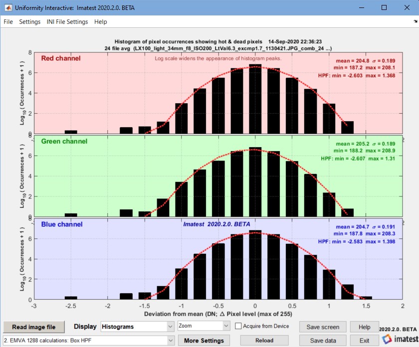
Standard histograms — illustrated in EMVA §8.4, Figure 13. Can be calculated for light or dark images. Here are two examples, without and with the box filter, which is recommended by EMVA 1288 (§C.5) for removing low spatial frequency nonuniformities.

Proceed to the multi-image verification by clicking Analyze. In this window, be sure to select Read n >= 4 files for pixel-based temporal noise when performing analyses for EMVA1288. Select Yes to proceed.

The European Machine Vision 1288 standard (EMVA 1288) is designed to test several key qualities of linear image sensors, including linearity, sensitivity (quantum efficiency), noise, dark current, nonuniformities, and spectral sensitivity. Imatest 2020.2 and later performs a subset of these measurements, including temporal noise and spatial nonuniformities in flat-field images. Results including Photo Response Nonuniformity and Dark Signal Nonuniformity (PRNU or DSNU for light and dark (“lens cap on”) images, respectively), can be calculated from batches of flat-field images in the Uniformity and Uniformity Interactive modules.

Total spatial variance can be further decomposed into row, column, and pixel spatial variances, which is useful for characterizing row-to-row and column-to-column nonuniformities:

Note that PRNU/DSNU statistics require data from both light and dark sets of image data. To populate these statistics, select “Read image file” and repeat the analysis for a set of dark images (or light, if dark was calculated first). Both dark and light images must have the same size and type (monochrome, Bayer raw, or demosaiced) in order for DSNU/PRNU statistics to be computed.

A note on EMVA 1288 equations: Imatest does not currently use photometric units, such as K = Digital Number (DN) per electron; η = quantum efficiency; μp = mean number of photons per pixel; μe = mean number of electrons per pixel ( μe = η μp ). Imatest results are derived only from electrical measurements, therefore we are unable to follow the equations the standard exactly.

In the Uniformity or Uniformity Interactive More settings window, select EMVA 1288 calculations, Box filter. For Uniformity, select the plots.

Set the threshold for dark image classification in your INI settings. This functionality is available starting in Imatest 24.1 and allows the user to manually set the threshold used to classify “light” and “dark” images. The threshold is based on the normalized mean value of the input images, and is set to 0.08 by default. This means that the average digital count across all of the input images must be less than 8% of the maximum digital number in order to be classified as “dark”. In some instances, this threshold may be too low to classify a set of input images as intended. To adjust this threshold in the .ini file, go the the INI dropdown in the Imatest Main Window and select Open INI File.

These measurements are derived from the EMVA 1288 standard and have similar numerical results, but they are not strictly EMVA 1288-compliant because the methodology is different. A sensor Dynamic Range measurement, is also designed to give results comparable to EMVA 1288, and again, it’s far from compliant.

\(\displaystyle\mu_y = \frac{1}{MN}\sum_{m=0}^{M-1}\sum_{n=0}^{N-1}\langle y \rangle[m][n]\)      EMVA Linear Version 4.0 (34)

If possible, prior to acquiring the data, in the Settings dropdown menu, Signal averaging should be set to the desired number, and Calculate image^2 while averaging (which has the same function as Read n files … for EMVA-1288, above) should be checked. (This name may change.) It should be easy to repeat the data acquisition using the Acquire image (Read Image File) button on the bottom-left of the Uniformity Interactive window.

Several plots, selected in the Display dropdown window, contain EMVA 1288 results. These include Histograms, Accum. Histograms, V&H Spectrum, PRNU, DSNU & Hist, and Temporal noise image.

\(\displaystyle PRNU_{1288} = \frac{\sqrt{\langle s_{y.light}\rangle ^2 – \langle s_{y.dark}\rangle ^2 } } { \langle \mu_{y.light}\rangle – \langle \mu_{y.dark}\rangle}\)

In the More settings window, EMVA 1288 should be set to EMVA 1288 calculations: Box filter. The 5×5 Box filter is a highpass filter, described in §C.5, designed to suppress low-frequency spatial variations.

Using Flatfield, Part I  |  Using Flatfield, Part 2  |  Using Flatfield Interactive  |  Temporal noise  EMVA 1288 — Machine Vision Test Standard  |  Flatfield Statistics based on EMVA 1288  |  Color/Tone/eSFR ISO Noise

When both light and dark data have been loaded and analyzed, the PRNU/DSNU statistics will populate in the displayed results table:

Accumulated histograms — illustrated in EMVA §8.4, Figure 14. We are not sure how to use them. Does not contain EMVA required results.

The full EMVA 1288 Photo Response Nonuniformity (PRNU1288)  measurement uses a set of light images, designated by the subscript 50 or light, and a set of dark images, designated by the subscript dark. When a set of images is run, results are temporarily stored in imatest-v2.ini. PRNU1288 is only calculated when both light and dark are available.

The equations below represent actual Imatest calculations, which are intended to be equivalent to the standard measurements. We will try to follow some EMVA 1288 notation. μ represents the mean; s represents spatial standard deviations; σ represents temporal standard deviations.

For saved image files, select a group of L (light or dark) files, and then select the Flat Field analysis, and choose the desired Interactive or Auto (batch) option.

This will open your existing .ini configuration file in a text editor. If starting from the default .ini or if you have not previously run a Flat Field analysis, you will need to add the [flatfield] section and threshold_Lt_Dk_pct_0_1 manually, as shown below.

This equation could be slow and tedious to evaluate, but there is a shortcut, described in the Wikipedia Variance page. In Wikipedia’s notation, \(E(x) = E[(x-E[x])^2] = E[x^2]-E[x]^2\). In the EMVA notation,

Spatial nonuniformity s is the standard deviation of μy, such that the overall spatial variance, \(\displaystyle s_y^2 \),  is equal to the mean.

Noise from a real image, shown with increased contrast; 4 display pixels per image pixel. Some 8×8 blocking from (low quality) JPEG processing  is visible.

And likewise, the row spatial variance is computed from average column of the combined image. \(\displaystyle s_{y.row}^2, s_{y.col}^2\), and \(\displaystyle s_{y.pixel}^2\) are solved using a system of equations defined in Section 4.3 of the EMVA Linear Version 4.0.

\(\displaystyle \sigma_{y}^{2}=\frac{1}{2MN}\sum_{M=0}^{M-1}\sum_{N=0}^{N-1}(y[0][m][n]-y[1][m][n])^{2}-\frac{1}{2}(\mu[0]-\mu[1])^{2} \)    EMVA Linear Version 4.0 (18)

\(\displaystyle s_{y.col}^2=\frac{1}{N}\sum_{n=0}^{N-1}(\mu_y[n]-\mu_y)^2- s_{y.pixel}^2/M-\sigma_{y}^{2}/(LM)\)    EMVA Linear Version 4.0 (39)

DSNU

Temporal noise image — Temporal noise power (variance) σ2 and RMS voltage σ as defined in the equations in the green box (above) are calculated for each pixel, i.e., they are images. For the flat-field images used in the EMVA calculations, temporal noise images are not of much interest, but they are of great interest for test chart images because they show how image processing varies across the image field. (When bilateral filtering is applied, noise is typically larger near edges than in smooth areas.) See Temporal noise for more details.

There are two ways of measuring temporal noise. Method 1 subtracts two images acquired under identical conditions, then divides by √2. Method 2 requires a large number of images. This method is used by the EMVA calculation because multiple images are also required to obtain spatial nonuniformity.

For direct data acquisition, select the acquisition device with the Device Manager, which can be opened from the Settings dropdown menu in the Imatest main window, the Data tab in the box on the right, or the Uniformity Interactive Settings window. When you’ve made the selection, press  Save .

Photograph a flat field, which is typically a highly even light source, such as a non-flickering LED lightbox. For the bright images, if exposure control is available, choose an exposure to linear images are about 50% of the maximum level (this would be about 73% of maximum for a gamma = 2.2 color space).

This “measured” spatial variance can then be corrected for the residual variance of the temporal noise by subtracting \(\displaystyle\sigma_s^2/L \):