For the same compound, there is a preset wavelength where the optimal wavelength is found; select this mode and record the wavelength.

In a conventional light source such as a gas discharge lamp, photons are generated by electronic transitions in the atoms of the gas. These transitions have a duration of the order of \(10^{-8}\) to \(10^{-9} \mathrm{~s}\). Because the emitted wave trains are finite, the emitted light does not have a single frequency; instead, there is a band of frequencies around a centre frequency. This spread of frequencies is called the natural linewidth. Random thermal motions of the molecules cause further broadening due to the Doppler effect. In addition, the atoms undergo collisions that interrupt the wave trains and therefore further broaden the frequency spectrum.

Absorptionspectra

To do this, you will use the spectrophotometry virtual lab by Gary L. Bertrand.  In this virtual experiment, you will prepare a Beer’s Law plot for one of the two solutes and then study the absorption spectrum.  This simulates the operation and use of an old Spectronic 20D spectrophotometer.

The LibreTexts libraries are Powered by NICE CXone Expert and are supported by the Department of Education Open Textbook Pilot Project, the UC Davis Office of the Provost, the UC Davis Library, the California State University Affordable Learning Solutions Program, and Merlot. We also acknowledge previous National Science Foundation support under grant numbers 1246120, 1525057, and 1413739. Privacy Policy. Terms & Conditions. Accessibility Statement. For more information contact us at info@libretexts.org.

When dealing with coherence one has to consider fields that consist of a range of different frequencies. Let \(\mathcal{U}(\mathbf{r}, t)\) be the real-valued physical field component. It is always possible to write \(\mathcal{U}(\mathbf{r}, t)\) as an integral over time-harmonic components: \[\mathcal{U}(\mathbf{r}, t)=\operatorname{Re} \int_{0}^{\infty} A_{\omega}(\mathbf{r}) e^{-i \omega t} \mathrm{~d} \omega, \nonumber \] where \(A_{\omega}(r)\) is the complex amplitude of the time-harmonic field with frequency \(\omega\). When there is only a certain frequency band that contributes, then \(A_{\omega}=0\) for \(\omega\) outside this band. We define the complex time-dependent field \(U(\mathbf{r}, t)\) by \[U(\mathbf{r}, t)=\int_{0}^{\infty} A_{\omega}(\mathbf{r}) e^{-i \omega t} \mathrm{~d} \omega . \nonumber \]

Waterabsorptioncoefficient

Based on this, the molar absorptivity can be found as the slope of the Beer’s Law plot is equal to . The molar absorptivity of the compound at a given wavelength can therefore be solved as the slope if you know what the pathlength is; most of the time, we use cuvettes with a path length of 1 cm.

Given the molar absorptivity, we can determine the concentration of an unknown solution of the same compound[4] by measuring the absorbance of the sample at the same wavelength as was done for the standard solutions. Given this, we can solve Beer’s Law to find the concentration of the substance.

Quasi-monochromatic field. If the width \(\Delta \omega\) of the frequency band is very narrow, we speak of quasi-monochromatic flight. In the propagation of quasi-monochromatic fields, we use the formula for time-harmonic fields at the centre frequency \(\bar{\omega}\). The quasi-monochromatic assumption simplifies the computations considerably. Nevertheless, most of the treatment that follows is more general and does not assume that the field is quasi-monochromatic.

AIn this experiment, we will work on relating how light is absorbed by a solution with the concentration of a solute that absorbs light, and how this can be used to determine the concentration of a solute.

Measure the absorbance at a number (at least 5) of concentrations and record your measurements.  What happens qualitatively to the amount of light that shines through the cuvette?

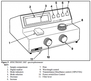
(1)   Note that is a dimensionless quantity.  The absorbance of a substance is typically measured using a spectrometer (of which there are many models).  One can plot the absorbance of a solution or substance as a function of the wavelength (i.e. color), as shown in the example below. The absorption spectrum of methylene blue.  Source: Wikimedia The Color of a Sample and the Light Absorbed As you will see later when we discuss the electromagnetic spectrum,[2] there is a whole range of different colors which vary in the wavelength of the waves.  When light is absorbed, that color of light is therefore removed from what is transmitted. The visible spectrum of light. Color Wavelength (nm) violet 380-430 blue 430-500 cyan 500-520 green 520-565 yellow 565-580 orange 580-625 red 625-740 We will explore in this experiment how the color of a substance relates to the wavelength of light absorbed. Absorbance and Concentration: Beer’s Law As you may have seen before, as the concentration of a solute increases, the color is darker and the amount of light absorbed would have increased.  More quantitatively, it can be shown that  for a solution with a concentration (molarity, or any other unit) of , the absorbance is related to this by (2)   where is the path length (the thickness of the solution through which the light travels; this is typically reported in centimeters) and is the molar absorptivity[3] (with units of ). The molar absorptivity varies with wavelength, and is a property of a particular substance at a given wavelength. The molar absorptivity at a given wavelength can be found by producing a Beer’s Law plot. To do this, solutions of different concentrations of the compound being studied are prepared and their absorbances at the chosen wavelength are plotted (along the -axis) against the concentrations of these solutions (along the -axis). A Beer’s Law plot. Based on this, the molar absorptivity can be found as the slope of the Beer’s Law plot is equal to . The molar absorptivity of the compound at a given wavelength can therefore be solved as the slope if you know what the pathlength is; most of the time, we use cuvettes with a path length of 1 cm. Given the molar absorptivity, we can determine the concentration of an unknown solution of the same compound[4] by measuring the absorbance of the sample at the same wavelength as was done for the standard solutions. Given this, we can solve Beer’s Law to find the concentration of the substance. You should, however, be aware that Beer’s Law only works for relatively low concentrations. Beyond an absorbance of about , the equation breaks down and can no longer be applied. For this reason, concentrations in the experiment should be chosen to have absorbances that are high enough to have a reasonable absorbance, but below the threshold of . This technique is very widely used in experimental chemistry and is one of the primary ways, for example, by which proteins and nucleic acids are quantified in the biochemical laboratory. Procedures Part 1: Color and Concentration of a Solution In the first part of the experiment, you will use the PhET Beer’s Law simulation to study how the absorption and transmission of light relate to the color of the substance, as well as obtain a qualitative understanding of how the absorbance relates to the concentration.  Select the Beer’s Law option on the simulation. Each student will be assigned a specific compound to study by your instructor.  As part of this experiment, you will share your data with your lab group on the discussion forum.  Next week, you will answer additional analysis questions (as a 5-point assignment) that requires you to compare and contrast different spectra. Color and the Absorption Spectrum Experimental Procedure Select the solution you were assigned to study. Select variable under wavelength.  This allows you to change the wavelength of the light source. Record the initial wavelength, transmittance, and absorbance (you can switch between the latter two by varying the controls on the detector).  Look at the color of the light and record the color of light that is absorbed the most. Change the wavelength by approximately 20 nm, and repeat step 2 until you have recorded the entire spectrum. Data Analysis You are required to prepare two plots using Excel or another spreadsheet program: A plot of the transmittance vs wavelength A plot of the absorbance vs wavelength (absorption spectrum) The following video outlines how you would make such a plot. https://iu.mediaspace.kaltura.com/id/1_2qxoqnjp Save the Excel file as this will need to be uploaded to Canvas. Absorbance and Concentration Experimental Procedure For the same compound, there is a preset wavelength where the optimal wavelength is found; select this mode and record the wavelength. Measure the absorbance at a number (at least 5) of concentrations and record your measurements.  What happens qualitatively to the amount of light that shines through the cuvette? You are urged to select a range of absorbances such that the maximum absorbance is approximately 1. Analysis Make a Beer’s Law plot (absorbance vs concentration) Determine the molar absorbtivity of the solute.  The path length should be 1 cm. This is explained in the following video: https://iu.mediaspace.kaltura.com/id/1_bp1vjgma Like in the last exercise, you are required to share the Beer’s Law plot with your lab group. Part 2: Determining the Concentration of an Unknown While in the last part you were able to visualize the trends better and to investigate different solutions, it has two different flaws: It fails to demonstrate how you would actually use a spectrometer. It doesn’t teach you how to determine the concentration of a solute. To do this, you will use the spectrophotometry virtual lab by Gary L. Bertrand.  In this virtual experiment, you will prepare a Beer’s Law plot for one of the two solutes and then study the absorption spectrum.  This simulates the operation and use of an old Spectronic 20D spectrophotometer. On the right, you will see a rack with five test tubes. Tube 0 contains a blank solution (typically the solvent itself). Tubes 1, 2 and 3 are currently empty for you to put standard solutions in. Tube 4 contains either a red or a blue unknown. Tube 5 contains a mixture of the red and blue unknowns (we will not use this tube). In the actual laboratory, the vast majority of spectrophotometers today use square cuvettes that can be made of plastic, glass or quartz and are square in shape.  When you do the experiment in real life, you should (a) take care not to break glass/quartz cuvettes (these are very expensive and fragile), (b) make sure that the clear sides of the cuvettes are aligned with the light beam (usually there are two glazed sides), and (c) hold the cuvette on the glazed sides carefully with your fingers so fingerprints do not block the optical path. Calibrating the Spectrophotometer The Spectronic 20D is set such that the light path is blocked when there is no test tube in the light path.  This is a convenient way of calibrating the spectrometer so that 0% transmittance is a set level of light, accounting for the presence of stray light due to imperfections in the detector.  Similarly – and this is true of all spectrophotometers – you need to zero the spectrometer so that the absorbance of a solution with zero solute is read as zero. Please watch this video by Mark Garcia which demonstrates the use of the Spectronic 20D: Here is a diagram of the controls on this spectrophotometer: A labeled diagram of the Spectronic 20D. Note that controls 5, 6, 7, and 11 are not accessible in this simulation. The zero control and the transmittance/absorbance control knobs at the front will not give you exactly 0% transmittance/0 absorbance.  You are asked to set these to as close as possible.   Press the mode selection button and set it to TRANS.  This makes it set on % transmittance. Click on the power switch/zero control to turn on the spectrometer.  You then can see the wavelength on the left and the % transmittance on the right of the display.  By pressing on the left and right hand sides of the knob, tweak the zero control until the % transmittance is as close to zero as possible. Click on tube 0 (the blank).  The tube will be placed into the spectrometer.  Then, press the mode selection button and set it to ABS.  Use the transmittance/absorbance control to set the absorbance to as close to zero as possible.  Click on the cuvette holder to return the test tube to the test tube rack. Determining the Absorption Maximum In this part of the experiment, you will determine the wavelength where the absorption maximum occurs. Look at tube 4.  Make a tube with the same color as the unknown by clicking “up” on the arrow of that color.  This will fill a wash bottle with that liquid.  Fill tube 1 with that liquid by clicking on the wash bottle. Click on tube 1 (the unknown).  This will load the tube into the spectrophotometer. Press the scan button at the bottom.  This will produce the data needed to reproduce the absorption spectrum.  Record the wavelength (in nm) at the spectral peak. Using the wavelength control, change the wavelength to be that of the spectral peak. Remove the unknown tube. Re-calibrate the spectrometer as shown above now that you have the correct wavelength selected. Obtaining the Absorbance with Standard Solutions You are given two stock solutions: a 13.0 ppm stock solution of the red dye and a 10.0 ppm stock solution of the blue dye.  You are also given some solvent. You will need to use the appropriate standard solution for your unknown. In this part of the experiment, you will obtain data needed to create a Beer’s Law curve. Experimental Procedure To prepare solutions of different concentrations, you need to: Click on the up and down buttons to obtain the relevant amount of stock solution and solvent.  This will fill up the wash bottle with the relevant solution. Click on the wash bottle.  The next empty tube will be filled with the solution you prepared. Click on the tube to place the tube into the spectrophotometer.  Record the absorbance. Click on the “dump solutions” link at the right hand side if you have no more empty tubes left.  This will give you more empty tubes to work with. Data Analysis To obtain the concentration in a given test tube, you can solve for this using the equation you’ve seen in class for dilution calculations (3)   Here, instead of having concentrations in molarity, you will have concentrations in ppm.  This will affect the units on the -axis of your Beer’s Law plot, but not the actual calculations. The path length will be 1 cm.  You can use the same procedure as above to find the slope of the Beer’s Law plot. Find the Concentration of the Unknown Put tube 4 into the spectrophotometer and record the concentration.  You can then use the absorbance found and the slope of the plot from the previous part to find the concentration of the dye in ppm for your unknown. The discussion on this is rather complex and are well beyond the scope of this course; some discussion of this can be found in the CHEM-C 344 organic chemistry laboratory course. ↵Tro, Chemistry - A Molecular Approach (5th Ed), Ch. 8.2. ↵also called the molar extinction coefficient ↵In the same solvent, in principle, though the absorption spectrum doesn't vary too much as a function of solvent in many cases. ↵

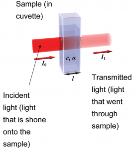
When light is incident on a sample, depending on the electronic structure of the molecule,[1] depending on the wavelength of the incident light some proportion of the light will be absorbed while the rest of the light is transmitted.

Visiblelightwavelength

Put tube 4 into the spectrophotometer and record the concentration.  You can then use the absorbance found and the slope of the plot from the previous part to find the concentration of the dye in ppm for your unknown.

Each student will be assigned a specific compound to study by your instructor.  As part of this experiment, you will share your data with your lab group on the discussion forum.  Next week, you will answer additional analysis questions (as a 5-point assignment) that requires you to compare and contrast different spectra.

Remark: The complex field \(U(\mathbf{r}, t)\) contains now the time dependence in contrast to the notation used for a time-harmonic (i.e. single frequency) field introduced in Chapter 2, where the time-dependent \(e^{-i \omega t}\) was a separate factor.

Click on the “dump solutions” link at the right hand side if you have no more empty tubes left.  This will give you more empty tubes to work with.

We use for the intensity again the expression without the factor \(1 / 2\) in front, i.e. \[I(\mathbf{r})=\left\langle|U(\mathbf{r}, t)|^{2}\right\rangle . \nonumber \] The time-averaged intensity has hereby been expressed in terms of the time-average of the squared modulus of the complex field.

The Spectronic 20D is set such that the light path is blocked when there is no test tube in the light path.  This is a convenient way of calibrating the spectrometer so that 0% transmittance is a set level of light, accounting for the presence of stray light due to imperfections in the detector.  Similarly – and this is true of all spectrophotometers – you need to zero the spectrometer so that the absorbance of a solution with zero solute is read as zero.

To understand coherence and incoherence, it is very helpful to use this model for the emission by a single atom as harmonic wave trains of thousands of periods interrupted by random phase jumps. The coherence time and the width \(\Delta \omega\) of the frequency line are related as

This technique is very widely used in experimental chemistry and is one of the primary ways, for example, by which proteins and nucleic acids are quantified in the biochemical laboratory.

To obtain the concentration in a given test tube, you can solve for this using the equation you’ve seen in class for dilution calculations

As you may have seen before, as the concentration of a solute increases, the color is darker and the amount of light absorbed would have increased.  More quantitatively, it can be shown that  for a solution with a concentration (molarity, or any other unit) of , the absorbance is related to this by

To quantify this, we note that – at a particular wavelength – given that the intensity of incident light is , the intensity of light that goes through the sample is ; the rest of this light is absorbed by the sample.  The absorbance of the light is related to the intensity of light transmitted by

We now compute the intensity of polychromatic light. The instantaneous energy flux is (as for monochromatic light) proportional to the square of the instantaneous real field: \(\mathcal{U}(\mathbf{r}, t)^{2}\). We average the instantaneous intensity over the integration time \(T\) of common detectors which, as stated before, is very long compared to the period at the centre frequency \(2 \pi / \bar{\omega}\) of the field (at least \(10^{5}\) times the period of the light). Using definition (5.2.6) and \[\mathcal{U}(\mathbf{r}, t)=\operatorname{Re} U(\mathbf{r}, t)=\left(U(\mathbf{r}, t)+U(\mathbf{r}, t)^{*}\right) / 2, \nonumber \] we get \[\begin{aligned} \left\langle\mathcal{U}(\mathbf{r}, t)^{2}\right\rangle &=\frac{1}{4}\left\langle\left(U(\mathbf{r}, t)+U(\mathbf{r}, t)^{*}\right)\left(U(\mathbf{r}, t)+U(\mathbf{r}, t)^{*}\right)\right\rangle \\ &=\frac{1}{4}\left\{\left\langle U(\mathbf{r}, t)^{2}\right\rangle+\left\langle\left(U(\mathbf{r}, t)^{*}\right)^{2}\right\rangle+2\left\langle U(\mathbf{r}, t)^{*} U(\mathbf{r}, t)\right\rangle\right\} \\ &=\frac{1}{2}\left\langle U(\mathbf{r}, t)^{*} U(\mathbf{r}, t)\right\rangle \\ &=\frac{1}{2}\left\langle|U(\mathbf{r}, t)|^{2}\right\rangle . \end{aligned} \nonumber \] where the averages of \(U(\mathbf{r}, t)^{2}\) and \(\left(U(\mathbf{r}, t)^{*}\right)^{2}\) are zero because they are fast-oscillating functions of time. In contrast, \(|U(\mathbf{r}, t)|^{2}=U(\mathbf{r}, t)^{*} U(\mathbf{r}, t)\) has a DC-component which does not average to zero.

While in the last part you were able to visualize the trends better and to investigate different solutions, it has two different flaws:

where is the path length (the thickness of the solution through which the light travels; this is typically reported in centimeters) and is the molar absorptivity[3] (with units of ). The molar absorptivity varies with wavelength, and is a property of a particular substance at a given wavelength.

The molar absorptivity at a given wavelength can be found by producing a Beer’s Law plot. To do this, solutions of different concentrations of the compound being studied are prepared and their absorbances at the chosen wavelength are plotted (along the -axis) against the concentrations of these solutions (along the -axis).

We first consider a single emitting atom. When collisions are the dominant broadening effect and these collisions are sufficiently brief, so that any radiation emitted during the collision can be ignored, an accurate model for the emitted wave is a steady monochromatic wave train at frequency \(\bar{\omega}\) at the centre of the frequency band, interrupted by random phase jumps each time that a collision occurs. The discontinuities in the phase due to the collisions cause a spread of frequencies around the centre frequency. An example is shown in Figure \(\PageIndex{1}\). The average time \(\tau_{0}\) between the collisions is typically less than 10 ns which implies that on average between two collisions roughly 150,000 harmonic oscillations occur. The coherence time \(\Delta \tau_{c}\) is defined as the maximum time interval over which the phase of the electric field can be predicted. In the case of collisions-dominated emission by a single atom, the coherence time is equal to the average time between subsequent collisions: \(\Delta \tau_{c}=\tau_{0}\).

Remark: In contrast to the time-harmonic case, the long time average of polychromatic light depends on the time \(t\) at which the average is taken. However, we assume in this chapter that the fields are omitted by sources that are stationary. The property of stationarity implies that the average over the time interval of long length \(T\) does not depend on the time that the average is taken. Many light sources, in particular conventional lasers, are stationary. (However, a laser source which emits short high-power pulses cannot be considered as a stationary source). We furthermore assume that the fields are ergodic, which means that taking the time-average over a long time interval amounts to the same as taking the average over the ensemble of possible fields. It can be shown that this property implies that the limit \(T \rightarrow \infty\) in (5.2.6) indeed exists.

As you will see later when we discuss the electromagnetic spectrum,[2] there is a whole range of different colors which vary in the wavelength of the waves.  When light is absorbed, that color of light is therefore removed from what is transmitted.

Here, instead of having concentrations in molarity, you will have concentrations in ppm.  This will affect the units on the -axis of your Beer’s Law plot, but not the actual calculations.

In the first part of the experiment, you will use the PhET Beer’s Law simulation to study how the absorption and transmission of light relate to the color of the substance, as well as obtain a qualitative understanding of how the absorbance relates to the concentration.  Select the Beer’s Law option on the simulation.

Note that is a dimensionless quantity.  The absorbance of a substance is typically measured using a spectrometer (of which there are many models).  One can plot the absorbance of a solution or substance as a function of the wavelength (i.e. color), as shown in the example below.

An intuitive way to think about these concepts is in terms of the ability to form interference fringes. For example, with laser light, which usually is almost monochromatic and hence coherent, one can form an interference pattern with clear maxima and minima in intensities (so-called fringes) using a double slit, while with sunlight (which is incoherent) this is much more difficult. Every frequency in the spectrum of sunlight gives its own interference pattern with its own frequency dependent fringe pattern. These fringe patterns wash out due to superposition and the total intensity therefore shows little fringe contrast, i.e. the coherence is less. However, it is not impossible to create interference fringes with natural light. The trick is to let the two slits be so close together (of the order of \(0.02 \mathrm{~mm}\) ) that the difference in distances from the slits to the sun is so small for the fields in the slits are sufficiently coherent to interfere. To understand the effect of polychromatic light, it is essential to understand that the degree to which the fields in two points are coherent, i.e. the ability to form fringes, is determined by the difference in distances between these points and the source. The distance itself to the source is not relevant. In the next sections we study these issues more quantitatively.

In the discussion so far we have only considered monochromatic light, which means that the spectrum of the light consists of only one frequency. Although light from a laser often has a very narrow band of frequencies and therefore can be considered to be monochromatic, purely monochromatic light does not exist. All light consists of multiple frequencies and therefore is polychromatic. Classical light sources such as incandescent lamps and also LEDs have relatively broad frequency bands. The question then arises how differently polychromatic light behaves compared to the idealised case of monochromatic light. To answer this question, we must study the topic of coherence. One distinguishes between two extremes: fully coherent and fully incoherent light, while the degree of coherence of practical light is somewhere in between. Generally speaking, the broader the frequency band of the source, the more incoherent the light is. It is a very important observation that no light is actually completely coherent or completely incoherent. All light is partially coherent, but some light is more coherent than others.

Since \(\lambda \omega=2 \pi c\), we have \[\frac{\Delta \lambda}{\bar{\lambda}}=\frac{\Delta \omega}{\bar{\omega}}, \nonumber \] where \(\lambda\) and \(\bar{\omega}\) are the wavelength and the frequency at the centre of the line. Hence, \[\Delta \ell_{c}=c \frac{2 \pi}{\Delta \omega}=2 \pi \frac{c}{\bar{\omega}} \frac{\bar{\omega}}{\Delta \omega}=\frac{\bar{\lambda}^{2}}{\Delta \lambda} \nonumber \]

You are given two stock solutions: a 13.0 ppm stock solution of the red dye and a 10.0 ppm stock solution of the blue dye.  You are also given some solvent.