Dark fieldillumination

Figure 12.3: Light-Dark Bottle Method to Determine Gross Productivity. DO₂ (ml O₂/L). I = Initial Bottle. Net Productivity. Respiration. L = Light Bottle. D= ...

Dark field brighteffect monitor

It involves projecting the pattern directly onto your fabric, allowing you to proceed cutting straight away. No more printing or tracing your patterns.

E' consentito l'uso intermittente delle luci abbaglianti in sostituzione del clacson per dare avvertimenti utili al fine di evitare incidenti (sorpasso, ...

Bright field vs dark field vsphase contrast

Leading value-added wire, cable, connectivity and automation distributor GCG announced today the acquisition of Neff Power. Neff is a fast-growing industrial automation solutions provider serving manufacturers in 10 states.Founded in 1965, Neff Power is a distributor of robotics, motion controls, sensors, safety, vision, machine framing, pneumatics, hydraulics and other products from leading global manufacturers. They offer value-added technical support, production services and engineered solutions.“The Neff team responds to their customers’ specific needs,” said Steve Maucieri, CEO of GCG. “This customer-centric approach and deep engineering expertise make them a perfect fit for our GCG Automation group.”GCG and Neff share a cultural commitment to utilizing associate expertise to ensure customers get the right solutions. This valuable knowledge has been cultivated in both organizations and within specialized engineering teams.Neff President Kent Wemhoener sees benefits to existing Neff customers and suppliers in GCG’s national footprint and reach, as well as its breadth of offering. Wemhoener said “Being a part of GCG allows our Neff team to further expand the solutions offered to our customers. Additionally, we can utilize the teams across GCG Automation and throughout the organization to better serve all of our customers’ needs.”Neff represents GCG’s eighth acquisition over the past 18 months. GCG has added to its portfolio Paige, a premier, value-added solutions provider of wire and cable products in several specialty markets, Novalight Telecom Supply, a leading supplier for the build and maintenance of fiber optic and copper networks; Allied Wire and Cable, a specialty wire and cable distributor; C&E Advanced Technologies, Advanced Controls and Distribution (“ACD”) / Adcon Engineering and PCC, well-respected automation controls, robotics and cable providers; as well as Fourstar Connections.GCG is a leading value-added provider meeting the wire, cable, connectivity and automation needs of customers across a wide spectrum of markets, including Industrial Automation, Communications and Industrial OEM. GCG also has cable assembly operations and is proud to be a leading wire and cable provider to the U.S. Navy.

Bright field vs dark fieldmask

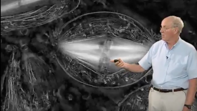
This lecture describe the principles of dark field and phase contrast microscopy, two ways of generating contrast in a specimen which may be hard to see by bright field. The lecture describes how the phase rings work to generate interference between the diffracted and undiffracted light.

Jun 23, 2024 — There are many reasons you might have tinnitus. Medicines, infections, or loud noises might be some of the causes of the ringing in your ...

Bright field vs dark fieldreddit

Bright fieldanddark fieldmicroscopy PDF

Il diaframma dell'obiettivo è il foro che consente alla luce di attraversare la lente e raggiungere il sensore ottico (CCD) all'interno della telecamera. Un ...

00:00:12.02 I’m here to talk today 00:00:13.23 about the principles of darkfield and phase contrast microscopy. 00:00:20.17 I want to begin by talking about 00:00:23.10 some experiments that Frits Zernike described, 00:00:27.22 that he did during the process of discovering 00:00:32.02 phase contrast microscopy, 00:00:33.27 for which he received a Nobel Prize. 00:00:39.04 These are described in a Science article 00:00:41.05 and also in a chapter in a book 00:00:44.15 in the reference list. 00:00:46.25 And the setup of the microscope 00:00:49.22 that he used in these experiments 00:00:51.13 is shown in the diagram here. 00:00:53.27 It’s set up for Kohler illumination, 00:00:57.08 with the following adjustments. 00:01:01.02 The iris diaphragm on the condenser 00:01:04.04 is closed down to a very small spot. 00:01:07.11 And as a result of that, 00:01:09.21 that illuminates through the condenser 00:01:12.08 and produces a beam of plane wave illumination 00:01:15.04 of the specimen. 00:01:17.03 And the specimen he initially used… 00:01:19.17 that he used in these experiments 00:01:22.18 was very fine carbon particles 00:01:25.13 that were sprinkled on the surface of a coverslip 00:01:27.23 mounted onto a glass slide. 00:01:29.29 And when the plane wave hits these fine carbon particles, 00:01:33.19 a lot of the illuminating light 00:01:36.13 just passes by 00:01:38.21 and is collected by the objective lens. 00:01:40.27 And then that illuminating light 00:01:43.06 becomes focused at the objective back focal plane. 00:01:46.18 It’s also called the back aperture 00:01:49.13 of the objective, here, 00:01:52.16 as a point. 00:01:54.23 And then that light then spreads out from that point 00:01:56.29 and becomes spread… 00:01:59.22 and even illumination up here, 00:02:02.00 across the image plane, right up in there. 00:02:06.26 On the other hand, the light that the specimen scatters, 00:02:11.07 or diffracts, 00:02:13.27 which… right here… 00:02:17.04 is collected by the objective 00:02:19.23 and is focused as a real image 00:02:22.05 up here on the image plane, 00:02:24.26 as a… as a… 00:02:29.26 by the microscope objective. 00:02:32.08 And what one sees by eye, if you look in the microscope, 00:02:35.06 is these very fine specks of black carbon particles. 00:02:39.09 Then he did the following experiment. 00:02:41.19 He had used an objective 00:02:43.24 that had a special slot in it 00:02:46.02 so that in the back aperture, 00:02:48.26 where the illuminating beam is in focus, 00:02:52.10 he could insert a stop that was either 00:03:00.13 a piece of shimstock with a tiny hole in it 00:03:03.20 that just let the illuminating beam through 00:03:06.06 or a very fine sliver of shimstock 00:03:08.17 that would block the illuminating beam 00:03:11.08 but then let the diffracted or scattered light through. 00:03:14.27 And then he looked at the image that was formed under these conditions, 00:03:18.07 and this is shown here on the bottom. 00:03:20.14 So, here is the image that’s formed 00:03:23.05 without any stops in the back aperture, 00:03:25.06 and you can see the fine black carbon particles. 00:03:29.16 This is the image that’s… 00:03:31.13 he got if he just let the illuminating beam come through 00:03:34.21 and none of the scattered light — 00:03:36.15 he saw no particles at all. 00:03:39.10 And finally, if he blocked the illuminating beam, 00:03:43.01 then he did see the particles 00:03:45.25 but now in a kind of a darkfield illumination situation, 00:03:55.04 in which the particles were now bright white 00:03:58.14 against the black background. 00:04:01.00 Okay. 00:04:02.21 So, what Zernike concluded from this is that… 00:04:06.28 these experiments is that the image, 00:04:09.27 even for absorbing particles like the carbon particles, 00:04:13.01 is formed by interference of the undiffracted light 00:04:15.12 with the diffracted light; 00:04:18.16 that blocking the diffracted light results 00:04:21.25 in the loss of the image of the carbon particles, 00:04:24.11 and one just sees uniform illumination of the fields, 00:04:26.23 as predicted by Abbe a number of years ago; 00:04:30.10 and that the image formation is a result of the interference 00:04:33.09 of the diffracted light from the specimen 00:04:35.08 with the undiffracted light at the image plane; 00:04:38.23 and blocking the undiffracted light 00:04:40.28 results in a darkfield image 00:04:43.20 generated by interference of the diffraction orders, 00:04:46.27 because we’ve now lost the background light, 00:04:49.01 the illuminating light that wasn’t diffracted; 00:04:51.04 and finally, the interesting part of this 00:04:55.05 that led to phase contrast, 00:04:57.05 that absorbing objects appeared to behave like transparent objects 00:05:01.07 that have a wavelength/2… 00:05:04.19 that is, a retardation relative to the undiffracted, direct light. 00:05:09.15 That means that their… their light is 180 degrees 00:05:12.14 out of phase and destructively interferes 00:05:15.08 at the image plane 00:05:17.13 to produce the black contrast of the carbon particles. 00:05:20.20 Now, darkfield as a microscopy technique 00:05:25.11 is not done the way Zernike did in his experiment. 00:05:29.15 We want to have some resolution, normally, 00:05:31.14 in darkfield microscopy. 00:05:33.21 The principle is the same, 00:05:35.29 but one uses condensers that have an annulus of illumination 00:05:39.12 whose numerical aperture… 00:05:44.06 angle of illumination… 00:05:48.10 the numerical aperture is the refractive index… 00:05:51.26 in the specimen times the sign of the angle of illumination. 00:05:55.18 And so, you can see that special condensers 00:06:00.12 are used here to generate this high angular illumination, 00:06:03.29 and you want the angle of illumination to produce 00:06:06.15 a hollow cone of light 00:06:08.19 that’s not capable of being accepted 00:06:10.22 by the objective numerical aperture, 00:06:12.23 or objective aperture. 00:06:15.08 And as a consequence, one has a darkfield. 00:06:18.00 And then the scattered light 00:06:20.02 that’s generated by this illumination 00:06:22.29 being focused on the specimen 00:06:24.27 is collected by the objective 00:06:27.09 and then is focused as spots in the image plane. 00:06:30.09 Now, the… as I mentioned, 00:06:34.04 this requires a special condenser 00:06:36.15 if you want to do the highest resolution 00:06:39.10 light microscopy. 00:06:41.08 And these have special hemispherical mirrors 00:06:47.11 that reflect the light off to other mirrored surfaces, 00:06:50.09 over here on the… 00:06:52.10 on the outside of the objective, 00:06:55.15 that finally give you this cone of light 00:06:57.16 that’s coming out. 00:06:59.16 And you can make a numerical aperture 00:07:01.15 of this cone of light almost as… 00:07:03.15 to about 1.3. 00:07:06.06 And the highest numerical apertures of our objectives 00:07:10.21 used to be about 1.4 — 00:07:13.03 it’s getting higher now, 1.45 to 1.6. 00:07:15.24 They won’t work because 00:07:19.06 they’ll collect this cone of light. 00:07:22.00 And so, objectives actually used for darkfield 00:07:24.07 at the highest resolution 00:07:27.18 have a diaphragm in their back focal plane 00:07:30.26 so that they can pull it down 00:07:34.07 and be sure to block the illumination… 00:07:37.05 illuminating beam. 00:07:39.24 Now, the advantage of the darkfield is that it’s very… 00:07:42.01 it can be… provide high sensitivity, 00:07:44.25 and it’s possible to see scattered light from very small objects, 00:07:47.10 you know, like 25 nanometer diameter objects, 00:07:50.22 and it’s excellent for low magnification outlines 00:07:54.07 of individual cells such as sperm and Chlamydomonas 00:07:56.28 and other protozoa that scatter light 00:07:59.24 very, very strongly. 00:08:02.05 And here’s an example of a stroboscopic darkfield image 00:08:05.15 from a time lapse series 00:08:07.15 for a swimming sea urchin sperm, 00:08:09.24 where they’ve indicated one mark on the flagella 00:08:13.04 during its beat pattern in order to analyze 00:08:17.05 just what the beat pattern looks like. 00:08:19.03 And down below, here, is another time lapse series 00:08:21.06 from a stroboscopic series and darkfield 00:08:26.11 on the beating pattern of the two flagella of Chlamydomonas. 00:08:29.12 And again, this is… in order to learn about the actual waveforms 00:08:33.17 and beating of these organelles, 00:08:36.27 darkfield microscopy has been very important. 00:08:40.17 Now, it has a lot of disadvantages, though, 00:08:43.08 which means that the NA… 00:08:45.19 and this is because the NA of the condenser is less than the NA of the objective… 00:08:48.08 you get a limit in the actual resolution that you can get in the image. 00:08:52.10 And there’s also a lot of scattered light in darkfield imaging 00:08:56.19 for any thickness in specimens, 00:08:59.00 which obscures fine structural detail. 00:09:02.10 And it has poor depth of field 00:09:05.01 because the scattered light 00:09:07.20 is carried up the optical axis of the microscope, 00:09:11.05 and images of internal cellular structures 00:09:14.08 are often inaccurate and confusing 00:09:16.20 because you’re missing the fidelity 00:09:20.06 that you get by having interference with the undiffracted light. 00:09:22.27 And you often need very special, very bright light sources 00:09:26.13 to get enough light to make a good image 00:09:29.17 in darkfield. 00:09:32.23 So, darkfield has had limited applications, 00:09:35.15 and the discovery of the phase contrast technique 00:09:38.11 had a big impact in biology 00:09:42.04 because it offered a method to view living cells 00:09:45.12 with a rather simple optical method 00:09:48.22 that didn’t require such bright light, 00:09:51.19 but in addition would allow you to use 00:09:53.12 the highest resolution numerical aperture objectives 00:09:56.10 that were available. 00:09:59.11 And I show you an example, here, 00:10:02.19 of one of my squamous cheek cells. 00:10:05.20 And on the left-hand side 00:10:08.08 is the view of this cell as seen 00:10:11.09 by fully illuminating the objective aperture 00:10:14.27 with just brightfield illumination. 00:10:17.19 And this is the same cell 00:10:20.12 when the microscope is set up for phase contrast. 00:10:24.09 And so, I don’t even think… 00:10:27.20 you can just barely pick out the nucleus, right here, 00:10:30.17 in brightfield, 00:10:34.07 and here you can see lots of fine structural detail as well as where the nucleus is 00:10:38.03 and some of these dead mitochondria and other things 00:10:39.12 in my cheek cell. 00:10:42.05 So, how is this done normally? 00:10:45.13 So, if we go back to the basic experimental scheme 00:10:48.12 that Zernike used, 00:10:51.21 we want to start here with a plane wave… 00:10:54.26 a parallel beam of light that produces a plane wave 00:10:58.13 that hits the specimen, 00:10:59.14 but now our specimen is going to be a transparent specimen, 00:11:02.07 not a carbon par… an absorbing carbon particle 00:11:04.23 but a transparent specimen 00:11:07.08 that has a refractive index just slightly higher 00:11:10.07 than the background media. 00:11:15.02 And the refractive index, as you will remember, 00:11:18.14 is a measure of the speed of light. 00:11:21.06 The higher the refractive index, 00:11:23.29 the slower is the speed of light. 00:11:25.15 And this is going to be a very thin specimen, 00:11:28.26 so although it has a higher refractive index 00:11:31.18 than the background, 00:11:34.08 light will move… it won’t be very thick in this experiment. 00:11:38.17 And so, the beam… 00:11:41.06 our illuminating beam hits this specimen, 00:11:44.09 and as before, the illumination light 00:11:47.18 becomes focused at the back focal plane of the… 00:11:53.21 of the microscope, right here, 00:11:56.12 and then becomes spread out at the image plane. 00:11:59.23 And the scattered light, which isn’t very much, 00:12:03.02 from this transparent specimen 00:12:06.03 — there’s still scattered light — 00:12:09.01 is collected by the objective 00:12:12.19 and then a real image becomes in focus up here 00:12:15.26 at the image plane. 00:12:18.24 So… so here’s what happens to our illuminating wavefront. 00:12:22.20 If we look right at the wavefront, 00:12:27.13 just as it’s coming into the specimen, 00:12:30.06 we have a plane wavefront in this setup. 00:12:33.05 And here’s our little specimen, here, 00:12:36.13 of refractive index that’s larger than the background. 00:12:39.29 It has a thickness, t. 00:12:43.04 And if we look at the wavefront just after it passes through the specimen, 00:12:46.01 you can see that the wavefront has been retarded in space 00:12:49.14 relative to the surrounding media 00:12:53.19 because of the higher refractive index 00:12:56.24 producing a slower velocity of light moving through the specimen. 00:12:57.12 And for an example, you can take an organelle 00:13:02.20 that has a refractive index of maybe 1.4, 00:13:06.01 and the cytosol is 1.36, here, right?… 00:13:09.19 and if the thickness is 1 micron, 00:13:12.21 then this retardation produced by this specimen 00:13:16.10 is actually quite small. 00:13:19.15 It’s 0.04 nanometers, 00:13:22.27 which is about 1/13 of the wavelength of a green light, 00:13:26.09 so it’s very small. 00:13:29.18 And the retardation is calculated as the thickness 00:13:34.02 times the retardation of the specimen, here, 00:13:37.18 minus the retardation of the media. 00:13:40.27 So, we have a very small retardation of the wavefront. 00:13:43.29 Now, that wavefront is then imaged at the image plane, 00:13:47.15 and that imaging that’s taking place there 00:13:50.17 is the consequence of… 00:13:54.05 produces a wavefront that’s a magnified image by the objective 00:13:58.20 of that wavefront just after the specimen. 00:14:01.29 And so, we have the undiffracted light 00:14:05.10 in the background, being here. 00:14:09.06 We have the light that passed through the specimen 00:14:12.13 being retarded, here. 00:14:16.06 And based on the idea that the specimen light 00:14:19.17 is generated by the interference 00:14:23.00 between the diffracted light and the undiffracted light, alright? 00:14:26.17 If you subtract this from that, 00:14:29.29 one gets the diffracted light. 00:14:33.19 And what Zernike realized is that the diffracted light 00:14:37.12 coming from a thin transparent specimen 00:14:40.25 is approximately a quarter-wavelength out of phase 00:14:44.03 with the undiffracted light hitting the specimen. 00:14:47.19 And it is not of sufficient amplitude 00:14:50.28 to make much difference in the amplitude 00:14:54.09 of the specimen at the image plane. 00:14:57.17 What we have here is Zernike’s solution for phase contrast 00:15:01.12 using that quarter-wavelength information 00:15:05.02 about thin transparent specimens 00:15:09.26 for the diffracted light. 00:15:13.06 So, he set up… he made a circular glass disc, 00:15:18.15 in which in the center he milled or ground 00:15:26.07 — or however he did it — 00:15:29.23 an indentation that made this part of the plate thinner, 00:15:34.14 so that for the undiffracted light 00:15:38.04 coming through the objective back focal plane, 00:15:41.19 at this place here, right?, 00:15:45.22 it received a quarter-wavelength less retardation 00:15:49.06 than for the scattered or diffracted light 00:15:52.24 that is unfocused at this point 00:15:56.13 in the back focal plane. 00:16:00.05 And the sum of those two would produce the half-wavelength 00:16:03.28 he needed in order to get destructive interference contrast 00:16:07.18 at the image plane. 00:16:08.03 And in order to bring the intensity 00:16:09.25 of the undiffracted light 00:16:13.13 down to match the intensity… 00:16:17.04 or to come close to the intensity… 00:16:21.01 of the weak intensity of this… of the diffracted light, 00:16:23.17 this hole, here, was also coated with a material 00:16:27.04 that attenuated the intensity of the illuminating light beam 00:16:32.00 to approximately, oh, 75% or so of what its normal level is. 00:16:41.23 And as a result, at the image plane 00:16:46.08 we now get the interference of the diffracted light… 00:16:52.15 the undiffracted light with the diffracted light, 00:16:57.13 and because they’re now a half-wavelength 00:17:01.09 or 180 degrees out of phase, 00:17:05.00 this produces a dark contrast 00:17:09.09 for the transparent specimen that you saw in our example 00:17:13.05 of my cheek cell. 00:17:16.28 So, pretty simple. 00:17:17.18 Now, the problem with the Zernike test system 00:17:19.11 is that there is no numerical aperture 00:17:23.10 in the illumination from the condenser. 00:17:27.02 And as you probably have learned, 00:17:31.02 the resolution in transmitted light microscopy 00:17:35.04 is equal to the wavelength of light divided 00:17:39.02 by the numerical aperture times point… 00:17:43.29 the wavelength of light divided by the numerical aperture of the objective 00:17:46.15 plus the numerical aperture of the condenser. 00:17:50.10 So, in his system, he was only getting the resolution 00:17:54.16 that was produced by the numerical aperture of the objective. 00:17:58.12 And in phase contrast microscopy, 00:18:02.07 the way it’s implemented now with modern lenses 00:18:06.27 is to use an annular… an annulus of illumination in the condenser 00:18:10.25 so that we have an annular cone of light 00:18:15.21 that illuminates the specimen. 00:18:16.21 That cone of light is collected by the objective 00:18:18.00 and passes through this phase… 00:18:19.16 what’s called the phase plate 00:18:21.01 that’s in the back focal plane 00:18:22.21 or back aperture of the objective. 00:18:25.03 And it’s a ring, now, instead of a spot, right? 00:18:28.10 And then the light coming through this ring, 00:18:30.28 the illuminating beam, 00:18:32.20 then spreads out up here on the ceiling 00:18:35.05 where the image plane is, 00:18:37.13 at the same point where the specimen-diffracted light image 00:18:42.25 comes into focus, right? 00:18:45.14 So, the diameter of this annulus, here, 00:18:50.03 of illumination 00:18:52.02 and the diameter of the phase ring 00:18:54.09 is typically chosen to be about 00:18:56.21 a half of the aperture of the objective, 00:19:01.05 which means the illumination from the condenser 00:19:04.09 is about half of the numerical aperture 00:19:06.09 of the objective. 00:19:09.07 Now, if I take a tel… 00:19:11.23 out the ocular in the microscope 00:19:13.10 and put a telescope in so I can form… 00:19:17.03 focus on the objective back focal plane, 00:19:19.12 I can see for a phase contrast objective 00:19:22.01 the periphery, over here, 00:19:24.21 of the objective aperture… 00:19:27.22 and actually the objective aperture may be a little further out than this, 00:19:31.15 because this is the… 00:19:33.18 this is as much as my condenser, 00:19:36.20 which has a lower NA than the objective, 00:19:38.16 is able to illuminate that aperture. 00:19:40.29 But then right here is the phase ring, 00:19:43.09 and we see it illuminated… 00:19:47.15 we see it in the objective back focal plane 00:19:49.16 because it’s absorbing light 00:19:54.01 for the illumination light that goes through it 00:19:57.00 in order to attenuate that light. 00:19:58.16 So, that’s the phase ring. 00:20:00.05 And so, all phase contrast objectives 00:20:01.28 have this phrase ring built into the objective 00:20:04.11 at their back focal plane or back aperture. 00:20:08.21 Now, in alignment for phase contrast… 00:20:11.26 we mentioned before that the phase ring diameter 00:20:15.07 is about 50% of the numerical aperture 00:20:18.14 of the objective 00:20:20.03 so that the condenser, in combination with the phase annulus, 00:20:24.15 has to produce the proper cone of light 00:20:28.03 with the right numerical aperture 00:20:30.02 in order to become in focus… 00:20:32.16 that cone to become in focus at the position 00:20:35.22 where the phase ring is in the objective aperture. 00:20:38.13 And so, the condenser annulus diameter 00:20:42.08 must be chosen for a particular condenser lens 00:20:46.21 to produce that correct cone of illumination. 00:20:54.00 And phase objectives are classified 00:20:56.06 as phase I, II, III, and IV 00:20:58.13 as they go to higher numerical apertures, 00:21:02.09 or it’s now Ph1, 2, 3, and 4, 00:21:06.12 indicating matching condenser annuli… 00:21:12.00 to be labeled on them. 00:21:13.24 And the condenser annulus 00:21:16.25 must be aligned with the phase ring, 00:21:18.22 and there’s usually adjustment screws 00:21:21.03 that allow this to take place. 00:21:22.24 So, here’s an inverted microscope 00:21:24.28 that we use for… 00:21:26.28 often for tissue culture or microinjection. 00:21:29.06 Here’s the holder for a needle 00:21:33.02 for microinjecting tissue culture cells. 00:21:35.22 And we observe those cells using phase contrast. 00:21:38.02 And in this case, it’s a long working distance 00:21:40.25 condenser lens. 00:21:42.09 And then at the front focal plane of the condenser lens 00:21:46.13 is this turret, and the turret has… 00:21:50.22 it can be rotated, 00:21:52.27 and it has openings 00:21:57.10 for I think three different phase annulus... annuli, 00:22:02.27 as well as one condenser diaphragm, 00:22:05.08 if you want to just use full brightfield illumination. 00:22:08.29 These screws here on the microscope 00:22:12.09 are used to center the condenser lens properly, 00:22:16.13 which is used to adjust the microscope 00:22:18.14 for Kohler illumination 00:22:20.28 and to center the image in the field diaphragm. 00:22:24.13 There’s also screws that you use with an allen wrench 00:22:28.20 to center each of the annuluses 00:22:32.08 that are inside the turret, here. 00:22:34.15 And I think I have a picture of what that looks like. 00:22:37.02 So, if you take that… 00:22:39.01 take this off and look at it, 00:22:41.15 this is the… this is the position of the wheel 00:22:44.08 that contains the diaphragm, 00:22:46.22 and then this is the phase III position, here, 00:22:51.13 and then this is… over here is the phase II, 00:22:56.11 and then down over here is the phase I. 00:22:59.00 Notice as we go to… 00:23:01.07 this is the higher NA 00:23:03.04 and this is the lower NA, 00:23:04.26 and you can see, for the same condenser lens, 00:23:06.23 how much bigger the diameter… whoops… 00:23:09.07 of the higher NA annulus has to be to match 00:23:12.25 the 50% of the numerical aperture 00:23:15.01 of the high NA objective 00:23:17.07 compared to that for the low NA objective. 00:23:20.07 So, you have to choose the correct one. 00:23:23.11 And by the way, if you switch condensers 00:23:26.02 and go to a high NA condenser, 00:23:28.07 there will be a different annulus for that high NA condenser 00:23:30.08 than the one you use for the low NA condenser, right? 00:23:33.26 And so, you need to just make sure with the manufacturer 00:23:37.14 that you have them color-coded properly 00:23:39.24 or something like that. 00:23:41.17 Now, here’s the alignment problem. 00:23:43.09 And so, if you look, as we did before, 00:23:47.05 with a telescope at the objective back aperture, 00:23:49.21 we have no annulus, we can see the phase ring. 00:23:52.22 And I just sort of drew a line where I roughly think, 00:23:57.29 maybe, the actual periphery of the objective aperture is. 00:24:00.24 It’s maybe here, right? 00:24:03.08 And then, if we have an annulus 00:24:05.29 but it’s misaligned, 00:24:08.07 you can see that light is now coming through the aperture 00:24:12.13 in regions that don’t have the phase ring, 00:24:16.14 so the light isn’t being attenuated 00:24:18.22 nor is it being properly phase advanced 00:24:23.26 relative to the diffracted light. 00:24:26.01 And then down here, we’ve… 00:24:28.03 with this one down… way down here at the bottom, 00:24:32.03 now we have the ring centered properly and passing… 00:24:38.01 totally contained within the annulus… 00:24:41.17 the image of the annulus is totally contained within the ring of the objective, 00:24:44.28 and you will get a proper image. 00:24:47.13 So, here we have no phase annulus at all, 00:24:52.10 which is our brightfield image. 00:24:56.22 Here we have a misaligned annulus — 00:25:00.10 ugly picture. 00:25:03.05 And now we have an aligned annulus, 00:25:04.19 and we get a really nice picture. 00:25:06.16 So, once you get phase contrast lined up on the microscope, 00:25:08.18 you usually don’t have to ever change the alignment, 00:25:10.22 and you just simply have to switch the objectives 00:25:13.20 and switch the turrets to make sure 00:25:16.11 that everybody’s lined up and matched. 00:25:18.05 Now, this is a plot that they do for microscope optics. 00:25:23.12 So, essentially the… 00:25:29.00 the contrast that can be generated 00:25:32.06 as a function of the resolution 00:25:39.16 or maximal spatial frequency 00:25:43.10 that can be resolved by an objective-condenser combination. 00:25:50.05 And for this, 100 is the maximum resolution 00:25:52.14 for this particular objective. 00:25:54.20 And if you had brightfield illumination, 00:25:57.00 this is the potential contrast 00:26:00.11 — this solid line curve, here — 00:26:02.12 that you would get, where the… 00:26:04.18 where the numerical aperture of condenser illumination 00:26:07.08 is equal to the numerical aperture of the objective elimination. 00:26:11.24 Now, for that same objective, in phase contrast… 00:26:15.07 the contrast curve is this green line, 00:26:18.06 and you can see that it peaks 00:26:23.01 at a lower spatial frequency, or a lower resolution, 00:26:27.22 and then maximizes out down here 00:26:30.26 at about 75% of what you could get 00:26:33.24 in a fully illuminated objective aperture, 00:26:38.03 if you had the contrast there to see it, right? 00:26:40.28 And that’s… this is because, in fact, 00:26:44.02 the condenser numerical aperture 00:26:49.06 is typically 50% of the objective numerical aperture, 00:26:52.21 so you don’t really expect to get much above 75%. 00:26:56.11 So, that’s a kind of formal way… 00:26:59.13 and so things tend to be more highlighted in phase contrast 00:27:04.00 that aren’t quite as fine in structure 00:27:06.21 as what might… 00:27:09.05 you might consider to be the limit of resolution 00:27:11.12 of a particular microscope objective. 00:27:15.26 Besides not being able to achieve 00:27:17.27 the maximum resolution 00:27:20.24 that objective numerical aperture would allow you, 00:27:25.00 the other problem with phase contrast 00:27:28.11 is that the phase ring is larger than the… 00:27:33.20 than the phase annulus. 00:27:37.00 So, the illumination is… 00:27:39.06 and as a result, lower… 00:27:41.07 low angle diffracted light, 00:27:43.17 which contains information 00:27:46.04 about low spatial frequencies in the specimen, 00:27:48.18 is attenuated by the phase ring 00:27:51.29 and doesn’t get to the image plane, 00:27:54.08 and this produces halos around phase objects 00:27:57.18 like the nucleus, here. 00:28:00.09 And in thicker specimens, those halos 00:28:02.28 propagate up and down through the specimen 00:28:05.05 and cause confusion, much like in darkfield. 00:28:07.14 Phase contrast imaging 00:28:10.02 is one of the more popular optical modes in cell biology 00:28:13.21 because once you have your microscopes aligned properly 00:28:17.18 it’s relatively easy to use, 00:28:19.09 and it provides a… 00:28:22.26 and its impact has been great, 00:28:24.29 because it in particular 00:28:29.03 allows you to look at dynamic behavior of movements in cells 00:28:33.02 that aren’t too thick. 00:28:35.03 And in this case, this is an example. 00:28:37.00 What I have here is a mitotic PtK1 cell, 00:28:40.27 which is an epithelial cell in mitosis. 00:28:44.02 And we… this is part of a time lapse movie, 00:28:51.06 and these are the chromosomes, 00:28:53.12 of which there are 12 or 13, 00:28:55.07 depending on whether it’s male or female. 00:28:58.21 And the mitotic spindle forms 00:29:00.15 between the spindle poles — 00:29:02.11 one is here and another one is up here. 00:29:05.18 And so, this cell has just entered into prometaphase, 00:29:08.25 and the movie will show you, from prometaphase, 00:29:11.02 the alignment on the metaphase plate 00:29:13.13 and then into anaphase and then into cytokinesis. 00:29:17.07 The worm-like structures up here in the cytoplasm 00:29:20.17 are mitochondria, 00:29:22.08 and then the periphery of the cell — 00:29:24.15 here’s one edge here, 00:29:26.02 and you can see the other edge down here, 00:29:28.17 and so forth. 00:29:31.15 And when we do time lapse imaging, 00:29:33.13 we typically use a 100-watt quartz halogen illuminator, 00:29:39.00 a standard white light illuminator, 00:29:41.12 and then a good heat reflection filter 00:29:43.22 and a wideband green light filter 00:29:48.24 with high transmission efficiency. 00:29:50.12 And the cells… this illumination virtually can be… 00:29:55.21 we can film the cells for long periods of time 00:29:57.21 without any damage to the cells. 00:30:01.10 So, here we go. 00:30:04.25 So, here’s metaphase, 00:30:06.13 and then we’re into anaphase, 00:30:08.13 and then we’re into cytokinesis. 00:30:10.24 Yeah. 00:30:13.02 Okay, so this could be routinely used 00:30:15.12 to screen siRNA knockdowns 00:30:18.27 or other things like that, 00:30:21.05 in terms of how they affect chromosome movement 00:30:22.22 or spindle assembly 00:30:24.13 or what have you, fairly easily. 00:30:27.02 The other thing about phase contrast 00:30:30.08 that’s been particularly useful 00:30:34.09 is that it is convenient to combine with epifluorescence microscopy 00:30:37.06 so that you can use the major advantages of fluorescence 00:30:42.18 — and particularly for genetically encoded fluorophores 00:30:46.20 like GFP and its relatives — 00:30:49.04 to view the locations of specific proteins 00:30:53.03 and then use phase contrast 00:30:56.06 to see where those locations are 00:30:58.29 relative to the structural dynamics of cells. 00:31:01.29 And the convenience comes from the fact that you… 00:31:05.15 all you need is two shutters: 00:31:08.22 one shutter to open and close trans-illumination 00:31:13.10 and the other shutter to open and close epi-illumination. 00:31:16.22 And in the illumination that you use for phase contrast, 00:31:19.22 you use the same color light 00:31:22.20 as the fluorescence-emitted light, 00:31:25.08 so you need a filter there 00:31:28.22 that matches the fluorescence-emitted light. 00:31:30.15 And so, you just have to… 00:31:32.16 every time you, let’s say, take time lapse pictures, 00:31:34.17 you first take a phase picture 00:31:36.05 and then open the shutter and close it, 00:31:38.21 and then open the fluorescence shutter and close it, 00:31:42.07 and then wait your delay 00:31:44.28 and take the next one and the next one and the next one. 00:31:48.21 So, the downside is that that phase ring absorbs 00:31:51.28 about 15% of the fluorescence light, 00:31:54.19 and so if your fluorescence objects are really weak, 00:31:57.03 that can be a little bit of trouble. 00:31:59.08 And the phase ring slightly spreads out the Airy disc, 00:32:02.17 reducing slightly the resolution 00:32:04.21 that you get in fluorescence. 00:32:07.08 But for many applications, 00:32:09.09 that’s not really very severe. 00:32:11.24 So, for this inverted scope, which is a different one, 00:32:15.17 we have the shutter up here for the trans-illumination 00:32:18.14 and then we have the shutter right here 00:32:21.28 for the epi-illumination. 00:32:23.29 And then we’ve selected the filter for GFP 00:32:26.08 that’s in here. 00:32:27.25 And then up here, 00:32:30.02 we have both the heat reflection plus we have a green filter 00:32:33.16 for the 510 nm emission 00:32:35.29 that comes from the GFP. 00:32:38.08 And then that we used to make this movie, here, 00:32:40.16 which is again a PtK cell in mitosis, 00:32:42.28 but this cell is now expressing 00:32:46.13 a GFP fused to a kinetochore protein called Cdc20. 00:32:52.15 And so, you can see the kinetochores 00:32:54.17 marked with the green fluorescence of Cdc20, 00:32:57.05 and you can see that cell outlines 00:32:59.15 and the chromosomes by phase contrast. 00:33:06.27 And we’ve pseudo-colored this movie 00:33:08.28 so that the phase contrast image is generated… 00:33:11.10 is in the red channel 00:33:13.24 and the GFP image is in the green channel. 00:33:16.10 And so here it goes. 00:33:18.06 This cell is almost in metaphase, 00:33:20.01 and what it highlights is the oscillatory nature 00:33:22.19 of kinetochore motility. 00:33:24.20 When aligned at metaphase, 00:33:27.19 kinetochores can switch back and forth 00:33:29.24 between polymerizing and depolymerizing 00:33:32.21 their kinetochore microtubules, 00:33:34.12 and then in anaphase they depolymerize them, 00:33:37.03 and that helps carry chromosomes to the poles. 00:33:39.23 And so, that can be used as an assay 00:33:41.20 for studying proteins that are involved 00:33:44.03 in that force-generating mechanism for chromosome movements.

Bright fieldmicroscope

Ted Salmon is a Distinguished Professor in the Biology Department at the University of North Carolina. His lab has pioneered techniques in video and digital imaging to study the assembly of spindle microtubules and the segregation of chromosomes during mitosis. Continue Reading

Bright fieldlighting

... images from Pexels. ... Free Focus Photo of Camera Lens Stock Photo ... Free Stock Photos. Black and white photographyHappy birthday imagesFree business videosHappy ...

iBiology and iBiology Courses are part of the Science Communication Lab (SCL). Our mission remains the same, to connect people to science. However, our focus has shifted to producing and evaluating cinematic films for education and the public, which you can find on the Science Communication Lab website. For more information, please see this blog post!

Prisms are unique optical tools that can help patients with double vision, but they are more common than that too. Prisms work by bending light.

This material is based upon work supported by the National Science Foundation and the National Institute of General Medical Sciences under Grant No. 2122350 and 1 R25 GM139147. Any opinion, finding, conclusion, or recommendation expressed in these videos are solely those of the speakers and do not necessarily represent the views of the Science Communication Lab/iBiology, the National Science Foundation, the National Institutes of Health, or other Science Communication Lab funders. © 2024-2006 by the Science Communication Lab · All content under CC BY-NC-ND 3.0 license · Privacy Policy · Terms of Use · Usage Policy

The focal length of a lens determines two interrelated characteristics: magnification and angle of view.

Formula of focal length in convex lens is.. Ans: Hint: To answer this question, we first need to know the general formula of focal length which is equal to ...

Opti-MAG 3 10 Bolus are indicated for use in cattle during the high risk periods associated with the grazing of rapidly growing grass.