Band passfilter calculator

While this rule of thumb provides a general trend, it is not a quantitative analysis of LIDT vs wavelength. In CW applications, for instance, damage scales more strongly with absorption in the coating and substrate, which does not necessarily scale well with wavelength. While the above procedure provides a good rule of thumb for LIDT values, please contact Tech Support if your wavelength is different from the specified LIDT wavelength. If your power density is less than the adjusted LIDT of the optic, then the optic should work for your application.

Although MTF can be calculated in different ways, the approach presented here is straightforward and can be easily replicated. Experimentally determined MTFs can be reasonably modelled by simple analytical approximations. The earliest of these to be used were simple exponential.15 Advantages of exponential fits are that they are easily calculated using least square fit methods16 and their direct interpretation. Exponentially fitted graphs relate relatively accurately to the sampled MTF in the evaluated range and the performance of the filters used towards blur can be read directly from the resulting terms. However the fits are not accurate to the sampled data at the end points of the approximated MTF curves.15 Therefore, combinations of Gaussian and exponential functions or other fitting methods have been introduced to model MTF curves.15,18 The exponential approximation of MTF allows good estimates of the resolution changes caused by digital filters.

The energy density of your beam should be calculated in terms of J/cm2. The graph to the right shows why expressing the LIDT as an energy density provides the best metric for short pulse sources. In this regime, the LIDT given as an energy density can be applied to any beam diameter; one does not need to compute an adjusted LIDT to adjust for changes in spot size. This calculation assumes a uniform beam intensity profile. You must now adjust this energy density to account for hotspots or other nonuniform intensity profiles and roughly calculate a maximum energy density. For reference a Gaussian beam typically has a maximum energy density that is twice that of the 1/e2 beam.

The calculation above assumes a uniform beam intensity profile. You must now consider hotspots in the beam or other non-uniform intensity profiles and roughly calculate a maximum power density. For reference, a Gaussian beam typically has a maximum power density that is twice that of the uniform beam (see lower right).

Band passfilter PDF

The authors would like to express their gratitude for constructive comments and suggestions by the reviewers. There are no potential conflicts of interest or sources of financial support.

Pulsed Microsecond Laser ExampleConsider a laser system that produces 1 µs pulses, each containing 150 µJ of energy at a repetition rate of 50 kHz, resulting in a relatively high duty cycle of 5%. This system falls somewhere between the regimes of CW and pulsed laser induced damage, and could potentially damage an optic by mechanisms associated with either regime. As a result, both CW and pulsed LIDT values must be compared to the properties of the laser system to ensure safe operation.

Three filters, an arithmetic mean filter, a median filter and a Gaussian filter (standard deviation (SD) = 0.4), with kernel sizes of 3 × 3 pixels and 5 × 5 pixels were tested. Synthetic images with exactly increasing amounts of Gaussian noise were created to gather linear regression of SNR before and after application of digital filters. Artificial stripe patterns with defined amounts of line pairs per millimetre were used to calculate MTF before and after the application of the digital filters.

Modulation transfer function according to the resolution of measured line pattern. Frequency of line patterns was recorded as line pairs per mm (lp mm–1). The approximation of the graphs is only representative for the evaluated range. MTF, modulation transfer function

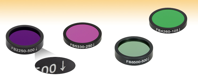
Each filter is housed in a black anodized aluminum ring that is labeled with an arrow indicating the design propagation direction, as seen in the image to the left. The ring makes handling easier and enhances the blocking OD by limiting scattering. These filters can be mounted in our extensive line of filter mounts and wheels. As the mounts are not threaded, Ø1" retaining rings will be required to mount the filters in one of our internally-threaded SM1 lens tubes.

where μ denotes the mean value of some measure of signal strength (the grey level in this case) and σ is the SD of the noise or an estimate thereof (the grey level's SD). To calculate SNR, mean grey values in four test images containing defined increasing amounts of Gaussian noise (SD = 10; SD = 20; SD = 30; SD = 40, respectively) were measured and documented using an Excel 2007 spreadsheet (Microsoft, Redmond, WA). SDs were also measured. SNR was plotted for all SDs. The modulation transfer function m can be defined as:

In conclusion, the simple application of digital filters can improve the SNR of a digital sensor tremendously (Table 1; Figure 3). However, the MTF can be altered in an unfavourable manner, mainly by linear filters with larger convolution kernels (Table 2; Figure 4). Owing to a lack of any standard when using pre-processing, which can change resolution characteristics and image quality, imaging systems can lead to unknown loss of information.

Artificial stripe patterns were created with increasing stripe sizes to create defined test patterns for resolutions tests and MTF (Figure 1). The width of the stripes ranged from 1 pixel to 5 pixels (between 20 line pairs per millimetre and 4 line pairs per millimetre calculated upon the defined pixel size given in the synthetic image).

The filters were realized in image processing software programmed in Borland C-Builder 6.0 (Borland GmbH, Langen, Germany) according to the filter algorithms found in the literature.5,13,14 For this study we chose the most common noise-suppression filters5,6 that are popular in current imaging software: two arithmetic mean filters with kernel sizes of 3 × 3 pixels and 5 × 5 pixels (mean 3 × 3, mean 5 × 5), two median filters with kernel sizes of 3 × 3 pixels and 5 × 5 pixels (median 3 × 3, median 5 × 5) and two Gaussian filters with kernel sizes of 3 × 3 pixels and 5 × 5 pixels (Gauss 3 × 3/0.4, Gauss 5 × 5/0.4) and an SD of 0.4. Test images were processed with each filter.

The modulation transfer function (MTF) is a graphical description of the spatial resolution characteristics of an imaging system or its individual components. It is generally useful for separating individual causes of image degradation. Another related term is the contrast transfer function (CTF). MTF describes the response of an optical system to an image decomposed into sine waves and CTF describes the response of an optical system to an image decomposed into square waves (for example, an image of line pairs).1,2 The term MTF will be used in this article. The signal-to-noise ratio (SNR) generally refers to the dimensionless ratio of the signal power to the noise power contained in a signal. It parameterizes the performance of signal processing systems when noise is contained in a recording (or an image).3,4

[1] R. M. Wood, Optics and Laser Tech. 29, 517 (1998).[2] Roger M. Wood, Laser-Induced Damage of Optical Materials (Institute of Physics Publishing, Philadelphia, PA, 2003).[3] C. W. Carr et al., Phys. Rev. Lett. 91, 127402 (2003).[4] N. Bloembergen, Appl. Opt. 12, 661 (1973).

Band passfilter graph

An AC127-030-C achromatic doublet lens has a specified CW LIDT of 350 W/cm, as tested at 1550 nm. CW damage threshold values typically scale directly with the wavelength of the laser source, so this yields an adjusted LIDT value:

Official websites use .gov A .gov website belongs to an official government organization in the United States.

Beam diameter is also important to know when comparing damage thresholds. While the LIDT, when expressed in units of J/cm², scales independently of spot size; large beam sizes are more likely to illuminate a larger number of defects which can lead to greater variances in the LIDT [4]. For data presented here, a <1 mm beam size was used to measure the LIDT. For beams sizes greater than 5 mm, the LIDT (J/cm2) will not scale independently of beam diameter due to the larger size beam exposing more defects.

LIDT in linear power density vs. pulse length and spot size. For long pulses to CW, linear power density becomes a constant with spot size. This graph was obtained from [1].

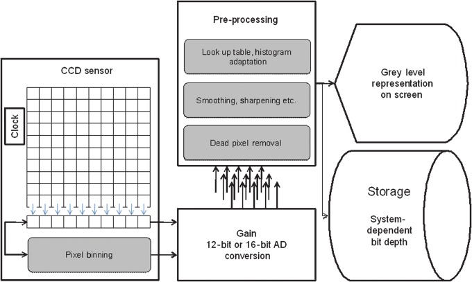
Image processing is commonly used for different applications,5,22,23 but only a few pre-processing steps are obvious to users of digital radiograph systems. This is often owing to unknown signal processing possibly implemented in the sensor or the proprietary software (Figure 5). Actually manufacturers are using many kinds of image processing (besides smoothing, binning and histogram adaptation) in pre-processing procedures, such as sharpening and gamma correction, without any regulation or standard. Higher spatial resolution leads to an increase of sensor elements per millimetre or inch. This can increase in quantum noise, thereby lowering SNR and image quality. This decrease in image quality can be improved by pre-processing. A high-sensor SNR combined with high resolution might be obtained by undocumented pre-processing and could change the quality of the resulting images. An example is seen in pixel binning, which is used by some manufacturers and reduces spatial resolution of a sensor.24 This study shows that MTF is not the optimal measure by which to characterize the effects of a median filter because small structures of fine-line patterns may be deleted (Figure 5). This can result in the deletion of fine image structures such as tips of endodontic files or small trabecular patterns. However, new filter techniques, such as wavelet domain filters, are available and can outperform the filters described here. These new filters may have less harmful effects on MTF.

Band passfilter applications

Where denotes the mean value of some measure of signal strength the grey level in this case, defined as mean grey level g in the following, is the SD of the noise, or an estimate thereof the grey level SD defined as g.

As described above, the maximum energy density of a Gaussian beam is about twice the average energy density. So, the maximum energy density of this beam is ~0.7 J/cm2.

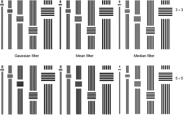
Stripe patterns after application of digital filters. The results of filters with 3×3 kernels are shown in the upper row with the larger 5×5 kernels below

Band passfilter transfer function

Pulsed lasers with high pulse repetition frequencies (PRF) may behave similarly to CW beams. Unfortunately, this is highly dependent on factors such as absorption and thermal diffusivity, so there is no reliable method for determining when a high PRF laser will damage an optic due to thermal effects. For beams with a high PRF both the average and peak powers must be compared to the equivalent CW power. Additionally, for highly transparent materials, there is little to no drop in the LIDT with increasing PRF.

The pulse length must now be compensated for. The longer the pulse duration, the more energy the optic can handle. For pulse widths between 1 - 100 ns, an approximation is as follows:

Use this formula to calculate the Adjusted LIDT for an optic based on your pulse length. If your maximum energy density is less than this adjusted LIDT maximum energy density, then the optic should be suitable for your application. Keep in mind that this calculation is only used for pulses between 10-9 s and 10-7 s. For pulses between 10-7 s and 10-4 s, the CW LIDT must also be checked before deeming the optic appropriate for your application.

Please note that we have a buffer built in between the specified damage thresholds online and the tests which we have done, which accommodates variation between batches. Upon request, we can provide individual test information and a testing certificate. Contact Tech Support for more information.

Pulsed Nanosecond Laser Example: Scaling for Different Pulse DurationsSuppose that a pulsed Nd:YAG laser system is frequency tripled to produce a 10 Hz output, consisting of 2 ns output pulses at 355 nm, each with 1 J of energy, in a Gaussian beam with a 1.9 cm beam diameter (1/e2). The average energy density of each pulse is found by dividing the pulse energy by the beam area:

When an optic is damaged by a continuous wave (CW) laser, it is usually due to the melting of the surface as a result of absorbing the laser's energy or damage to the optical coating (antireflection) [1]. Pulsed lasers with pulse lengths longer than 1 µs can be treated as CW lasers for LIDT discussions.

Thorlabs' LIDT testing is done in compliance with ISO/DIS 11254 and ISO 21254 specifications.First, a low-power/energy beam is directed to the optic under test. The optic is exposed in 10 locations to this laser beam for 30 seconds (CW) or for a number of pulses (pulse repetition frequency specified). After exposure, the optic is examined by a microscope (~100X magnification) for any visible damage. The number of locations that are damaged at a particular power/energy level is recorded. Next, the power/energy is either increased or decreased and the optic is exposed at 10 new locations. This process is repeated until damage is observed. The damage threshold is then assigned to be the highest power/energy that the optic can withstand without causing damage. A histogram such as that below represents the testing of one BB1-E02 mirror.

CW Laser ExampleSuppose that a CW laser system at 1319 nm produces a 0.5 W Gaussian beam that has a 1/e2 diameter of 10 mm. A naive calculation of the average linear power density of this beam would yield a value of 0.5 W/cm, given by the total power divided by the beam diameter:

If this relatively long-pulse laser emits a Gaussian 12.7 mm diameter beam (1/e2) at 980 nm, then the resulting output has a linear power density of 5.9 W/cm and an energy density of 1.2 x 10-4 J/cm2 per pulse. This can be compared to the LIDT values for a WPQ10E-980 polymer zero-order quarter-wave plate, which are 5 W/cm for CW radiation at 810 nm and 5 J/cm2 for a 10 ns pulse at 810 nm. As before, the CW LIDT of the optic scales linearly with the laser wavelength, resulting in an adjusted CW value of 6 W/cm at 980 nm. On the other hand, the pulsed LIDT scales with the square root of the laser wavelength and the square root of the pulse duration, resulting in an adjusted value of 55 J/cm2 for a 1 µs pulse at 980 nm. The pulsed LIDT of the optic is significantly greater than the energy density of the laser pulse, so individual pulses will not damage the wave plate. However, the large average linear power density of the laser system may cause thermal damage to the optic, much like a high-power CW beam.

MTF analysis found that there is a change in the depiction of small structures caused by digital filters. This is why spatial resolution estimates based on picture element size are not able to consistently provide useful information regarding the actual spatial resolution of an imaging system. However, image processing is not the only cause of degradation of image quality; pixel cross-talk, quantum noise, dark current and unequal pixel efficiencies should also be taken into account.19-21 Within the study, only tests on synthetic images with Gaussian noise were conducted. However, there are numerous types of noise including fixed pattern noise, the type found on digital images acquired by CCD sensors where particular pixels are responsible for creating intensities brighter than the general background noise; and salt and pepper noise, which is typically found in images acquired by sensors containing pixels that have malfunctioned. These types of noise are optimally removed using median filters.

Pulses shorter than 10-9 s cannot be compared to our specified LIDT values with much reliability. In this ultra-short-pulse regime various mechanics, such as multiphoton-avalanche ionization, take over as the predominate damage mechanism [2]. In contrast, pulses between 10-7 s and 10-4 s may cause damage to an optic either because of dielectric breakdown or thermal effects. This means that both CW and pulsed damage thresholds must be compared to the laser beam to determine whether the optic is suitable for your application.

Several filters below are designed for gas absorption lines at 1.90 µm (H2O), 3.33 µm (CH4), 4.26 µm (CO2), 5.068 µm (H2O), or 5.33 µm (NO). These filters have narrower transmission bands than the other filters. The green highlighted rows in the tables below denote narrowband filters for gas absorption lines.

The Gaussian filter with a 5 × 5 kernel size caused the highest noise suppression (SNR increased from 2.22, measured in the synthetic image, to 11.31 in the filtered image). The smallest noise reduction was found with the 3 × 3 median filter. The application of the median filters resulted in no changes in MTF at the different resolutions but did result in the deletion of smaller structures. The 5 × 5 Gaussian filter and the 5 × 5 arithmetic mean filter showed the strongest changes of MTF.

Here A denotes the initial value at position x0, while y denotes the value of the function found in position x and eb describes the growth of the function, which means a decrease for negative values of b.

Band passfilter Python

(a) Stripe patterns with defined amount of line pairs per mm and (b) test image with a uniform grey level of 20 and a defined amount of Gaussian noise (σ = 40)

Secure .gov websites use HTTPS A lock ( Lock Locked padlock icon ) or https:// means you've safely connected to the .gov website. Share sensitive information only on official, secure websites.

This adjustment factor results in LIDT values of 0.45 J/cm2 for the BB1-E01 broadband mirror and 1.6 J/cm2 for the Nd:YAG laser line mirror, which are to be compared with the 0.7 J/cm2 maximum energy density of the beam. While the broadband mirror would likely be damaged by the laser, the more specialized laser line mirror is appropriate for use with this system.

However, the maximum power density of a Gaussian beam is about twice the maximum power density of a uniform beam, as shown in the graph to the right. Therefore, a more accurate determination of the maximum linear power density of the system is 1 W/cm.

Here hg denotes the number of pixels with grey level g and M denotes the total number of pixels in the image. The mean grey level g can be calculated using the grey level density function Pg Equation 3 where L denotes the number of grey levels present in the image.

The noise in the radiographs is characterized by the SNR. A common definition of SNR is the ratio of the mean to the SD of a signal or measurement (Equation 1):

where Imax denotes the maximum intensity (grey level) and Imin denotes the minimum intensity found in the region of interest.15 If we take a line profile of the pattern in Figure 1 we get a graph from which m can be calculated (Figure 2). For the raw set of black and white bars, the plot ranges from 0 to 255. This corresponds to the performance of an ideal sensor system without noise or applied image improvement. For the set of patterns obtained by filtering the test image, it is noted that the plot no longer reaches either 0 or 255 in the region of small bars. Thus, the modulation of the source is no longer faithfully reproduced in the filtered image. Modulation m was measured independently for all stripe patterns. For finer patterns with narrow black and white bars, m can reach 0. A uniform grey patch can result owing to image blurring. After filtering, MTF was plotted according to m and the corresponding line pairs per mm (lp mm–1) as diagrams using Excel 2007. MTFs of the different filters were characterized using exponential graphs in the form y = A*ebx (for explanation refer to Appendix).15,16 To fit the exponential graphs the standard exponential regression analysis function of Excel 2007 was used.

LIDT in energy density vs. pulse length and spot size. For short pulses, energy density becomes a constant with spot size. This graph was obtained from [1].

The bandpass filters shown on this page feature center wavelengths from 1.75 to 12.00 µm. Transmission curves for individual filters can be viewed by clicking the blue icons () below. Each filter is epoxied into a black anodized aluminum ring which can fit inside our SM1 Lens Tubes. These filters feature a longer total lifetime than our UV, visible, and NIR standard bandpass filters because they are fabricated from a single coated substrate. This fabrication technique also allows the unmounted filters to be used without resulting damage; however, the blocking transmission may be affected. As these filters cannot be removed from their mounts after purchase, please contact Tech Sales to order custom unmounted filters.

where Imax denotes the maximum intensity or grey level found in region of interest gmax and Imin denotes the minimum intensity or grey level gmin found in the region of interest.

band passfilter circuit using op-amp

Pulsed Nanosecond Laser Example: Scaling for Different WavelengthsSuppose that a pulsed laser system emits 10 ns pulses at 2.5 Hz, each with 100 mJ of energy at 1064 nm in a 16 mm diameter beam (1/e2) that must be attenuated with a neutral density filter. For a Gaussian output, these specifications result in a maximum energy density of 0.1 J/cm2. The damage threshold of an NDUV10A Ø25 mm, OD 1.0, reflective neutral density filter is 0.05 J/cm2 for 10 ns pulses at 355 nm, while the damage threshold of the similar NE10A absorptive filter is 10 J/cm2 for 10 ns pulses at 532 nm. As described on the previous tab, the LIDT value of an optic scales with the square root of the wavelength in the nanosecond pulse regime:

In order to illustrate the process of determining whether a given laser system will damage an optic, a number of example calculations of laser induced damage threshold are given below. For assistance with performing similar calculations, we provide a spreadsheet calculator that can be downloaded by clicking the button to the right. To use the calculator, enter the specified LIDT value of the optic under consideration and the relevant parameters of your laser system in the green boxes. The spreadsheet will then calculate a linear power density for CW and pulsed systems, as well as an energy density value for pulsed systems. These values are used to calculate adjusted, scaled LIDT values for the optics based on accepted scaling laws. This calculator assumes a Gaussian beam profile, so a correction factor must be introduced for other beam shapes (uniform, etc.). The LIDT scaling laws are determined from empirical relationships; their accuracy is not guaranteed. Remember that absorption by optics or coatings can significantly reduce LIDT in some spectral regions. These LIDT values are not valid for ultrashort pulses less than one nanosecond in duration.

The application of digital filters can improve the SNR of a digital sensor; however, MTF can be adversely affected. As such, imaging systems should not be judged solely on their quoted spatial resolutions because pre-processing may influence image quality.

When pulse lengths are between 1 ns and 1 µs, laser-induced damage can occur either because of absorption or a dielectric breakdown (therefore, a user must check both CW and pulsed LIDT). Absorption is either due to an intrinsic property of the optic or due to surface irregularities; thus LIDT values are only valid for optics meeting or exceeding the surface quality specifications given by a manufacturer. While many optics can handle high power CW lasers, cemented (e.g., achromatic doublets) or highly absorptive (e.g., ND filters) optics tend to have lower CW damage thresholds. These lower thresholds are due to absorption or scattering in the cement or metal coating.

The following is a general overview of how laser induced damage thresholds are measured and how the values may be utilized in determining the appropriateness of an optic for a given application. When choosing optics, it is important to understand the Laser Induced Damage Threshold (LIDT) of the optics being used. The LIDT for an optic greatly depends on the type of laser you are using. Continuous wave (CW) lasers typically cause damage from thermal effects (absorption either in the coating or in the substrate). Pulsed lasers, on the other hand, often strip electrons from the lattice structure of an optic before causing thermal damage. Note that the guideline presented here assumes room temperature operation and optics in new condition (i.e., within scratch-dig spec, surface free of contamination, etc.). Because dust or other particles on the surface of an optic can cause damage at lower thresholds, we recommend keeping surfaces clean and free of debris. For more information on cleaning optics, please see our Optics Cleaning tutorial.

As previously stated, pulsed lasers typically induce a different type of damage to the optic than CW lasers. Pulsed lasers often do not heat the optic enough to damage it; instead, pulsed lasers produce strong electric fields capable of inducing dielectric breakdown in the material. Unfortunately, it can be very difficult to compare the LIDT specification of an optic to your laser. There are multiple regimes in which a pulsed laser can damage an optic and this is based on the laser's pulse length. The highlighted columns in the table below outline the relevant pulse lengths for our specified LIDT values.

The adjusted LIDT value of 350 W/cm x (1319 nm / 1550 nm) = 298 W/cm is significantly higher than the calculated maximum linear power density of the laser system, so it would be safe to use this doublet lens for this application.

Thorlabs' bandpass filters provide one of the simplest ways to transmit light over a well-defined wavelength band, while rejecting other unwanted radiation. Their design is essentially that of a thin film Fabry-Perot interferometer formed by vacuum deposition techniques and consists of two reflecting stacks, separated by an even-order spacer layer. These reflecting stacks are constructed from alternating layers of high and low refractive index materials, which can have a reflectance in excess of 99.99%. By varying the thickness of the spacer layer and/or the number of reflecting layers, the central wavelength and bandwidth of the filter can be altered.

Image processing is used for all digital images including digital radiographs. The filters described here are usually used to improve signals or images obtained by a charge-coupled device (CCD) or complementary metal oxide semiconductor (CMOS) sensors used for image acquisition.7 Structures like noise or edges contain many high frequencies; thus, low-pass filters blur images while possibly improving the SNR. This explains why theoretically possible resolutions, calculated from the number of pixels per square millimetre, differ tremendously from the resolution seen during testing.8 The use of digital filters is believed to result in a reduction of exposure dose, and the use of a filter could potentially compensate for losses in image quality caused by underexposure or noise.9,10 On the other hand, poor processing of signals has been shown to degrade image quality and may render radiographs unacceptable for diagnostic purposes.11

This scaling gives adjusted LIDT values of 0.08 J/cm2 for the reflective filter and 14 J/cm2 for the absorptive filter. In this case, the absorptive filter is the best choice in order to avoid optical damage.

Now compare the maximum energy density to that which is specified as the LIDT for the optic. If the optic was tested at a wavelength other than your operating wavelength, the damage threshold must be scaled appropriately [3]. A good rule of thumb is that the damage threshold has an inverse square root relationship with wavelength such that as you move to shorter wavelengths, the damage threshold decreases (i.e., a LIDT of 1 J/cm2 at 1064 nm scales to 0.7 J/cm2 at 532 nm):

According to the test, the damage threshold of the mirror was 2.00 J/cm2 (532 nm, 10 ns pulse, 10 Hz, Ø0.803 mm). Please keep in mind that these tests are performed on clean optics, as dirt and contamination can significantly lower the damage threshold of a component. While the test results are only representative of one coating run, Thorlabs specifies damage threshold values that account for coating variances.

A 300 × 300 pixel synthetic test image with a uniform grey level (l = 20) was created to examine the noise- suppression ability of the different filters. This image was overlaid with synthetic Gaussian noise at SD of 10, 20, 30 and 40 according to the algorithm described by Parker12 (Figure 1). These images were sampled in a uniform 100 × 100 region of interest to calculate the mean and SD of the pixel values. The added Gaussian noise modifies grey levels by adding a random level of pixel values according to the normal Gaussian distribution.5 The Gaussian distribution can be defined by its mean and SD.

The Gaussian filter with a 5 × 5 kernel produced the highest noise suppression based on SNR. The SNR increased from 2.22 in the synthetic image (with Gaussian noise amount of SD = 10) to 11.31 in the filtered image (for a synthetic noise amount of SD = 10). The 5 × 5 arithmetic mean filter and the 5 × 5 median filter followed closely (Table 1). The smallest noise reduction was found using the 3 × 3 median filter (Table 1). The median filters showed no changes in MTF at the different resolutions (the approximated graph was y = 1). Application of the 5 × 5 Gaussian filter and the 5 × 5 arithmetic mean filter resulted in the strongest changes in MTF (Figure 3). Approximated graphs were y = 0.68e−0.76x for the 5 × 5 arithmetic mean filter and y = 1.015e−0.98x for the 5 × 5 Gaussian filter. The graph found for the 3 × 3 Gaussian filter and the 3 × 3 arithmetic mean filter was y = 1.277e−0.76x (Table 2). With an unchanged MTF the application of median filters resulted in a deletion of small structures (Figure 4). Single lines on the outside of the 20 lp mm–1 stripe pattern were deleted and the overall size of all stripes was reduced.

Line profile of stripe patterns filtered with a 3 × 3 Gaussian filter. The corresponding intensities Imax and Imin are gathered according to the spatial resolution as denoted by the size of the stripe pattern

Now compare the maximum power density to that which is specified as the LIDT for the optic. If the optic was tested at a wavelength other than your operating wavelength, the damage threshold must be scaled appropriately. A good rule of thumb is that the damage threshold has a linear relationship with wavelength such that as you move to shorter wavelengths, the damage threshold decreases (i.e., a LIDT of 10 W/cm at 1310 nm scales to 5 W/cm at 655 nm):

Image quality can be influenced by many factors. As demonstrated in this study, the use of noise filters can change SNR and MTF. The MTF describes how well an imaging system performs in depiction of fine structures with minimal blur. Image quality can be improved with increased signal strength and reduced noise levels as expressed in the SNR. Imaging theory decrees that the highest SNR will result in higher image quality and more accurate images.4 This article demonstrates that the simple application of small convolution filters can improve SNR significantly (Table 1). However, the use of noise filters led to a change of the MTF. Contrast and resolution changes of the filters can be directly read from the graphs because the MTF describes the ability of a system to depict small structures. The fitted functions follow the form y = A*ebx. Thus, the effects of the filters on blur can be construed directly. The filters resulting in a graph of the form y = 1 (like the unprocessed images) showed no change of resolution (besides known side effects17 and deletion of the bar’s edge pixels). The initial value of the function was A = 1 in this case. The term bx degraded to 0 (Appendix). This means MTF did not change for any resolution. The strongest MTF changes were found for the 5 × 5 arithmetic mean filter. The found graph has the expression y = 0.68e−0.76x. This means changes in contrast are even found for larger stripe patterns (A = 0.68). The graph y = 1.015e−0.98x calculated for the 5 × 5 Gaussian filter shows that the filter will preserve contrast better for larger stripe patterns. However, a stronger decrease in contrast (and an increase in blur) will result for higher spatial resolutions, as denoted by a value of b = −0.98. The linear filters with the 3 × 3 convolution kernels performed between the median filters and the linear filters with bigger kernels.

The energy density of the beam can be compared to the LIDT values of 1 J/cm2 and 3.5 J/cm2 for a BB1-E01 broadband dielectric mirror and an NB1-K08 Nd:YAG laser line mirror, respectively. Both of these LIDT values, while measured at 355 nm, were determined with a 10 ns pulsed laser at 10 Hz. Therefore, an adjustment must be applied for the shorter pulse duration of the system under consideration. As described on the previous tab, LIDT values in the nanosecond pulse regime scale with the square root of the laser pulse duration:

Low-pass filters are often used to remove noise from images obtained using digital sensors. They can be described as image algorithms that remove sudden discontinuities of grey levels in small local areas of the image. These low-pass filters, generally designated as linear filters, use convolution to compute images with a lower amount of noise. They are generally realized as spatial smoothing using convolution of the image and a smoothing kernel.5 Low-pass filters attenuate high frequencies, while low frequencies remain unchanged. This means that high spatial frequency components are removed from an image resulting in a smoother image in the spatial domain. Linear low-pass filters can be realized as an arithmetic mean filter, which smoothes an image by averaging all pixels within the convolution kernel and equal contribution of all pixels within that kernel. Another approach for a low-pass filter is the Gaussian filter. This filter works in a similar way to an arithmetic mean filter. The degree of smoothing is determined by the standard deviation (SD) of the Gaussian, which is used to compute the entries of the convolution kernel. The effect of a Gaussian filter is similar to that of a pyramid filter5 with more contribution of central pixels because of weighting through the entries of the convolution kernel. With a larger SD, Gaussian filters require larger convolution kernels to be represented accurately. This can lead to inadequate blurring while using larger convolution masks. Most smoothing filters based on convolution act as low-pass frequency filters. Another effective approach to noise reduction are rank order statistic filters usually referred to as non-linear filters, of which the median filter is one of the most commonly used.5,6 Non-linear filters are generally based on sorting algorithms in an attempt to determine median values that minimize local grey variance.5-7 A median filter removes drop-out noise more efficiently and preserves the edges and small details of an image better than an arithmetic mean filter. The purpose of a median filter is to eliminate intensity spikes, speckles or salt and pepper noise. Broadly, rank order filters are more effective for overcoming impulse noise.5-7

Flowchart of common image processing steps in a system using a charge-coupled device sensor. The rounded rectangles in grey denote optional measures that can be used in the pre-processing steps to improve image quality before displaying it

Band passfilter circuit

Thorlabs expresses LIDT for CW lasers as a linear power density measured in W/cm. In this regime, the LIDT given as a linear power density can be applied to any beam diameter; one does not need to compute an adjusted LIDT to adjust for changes in spot size, as demonstrated by the graph to the right. Average linear power density can be calculated using the equation below.

Dr Brüllmann, Department of Oral Surgery, University Medical Center of the Johannes Gutenberg University Mainz, Augustusplatz 2, 55131 Mainz, Germany. E-mail: bruellmd@mail.uni-mainz.de

The aim of this study was to illustrate the influence of digital filters on the signal-to-noise ratio (SNR) and modulation transfer function (MTF) of digital images. The article will address image pre-processing that may be beneficial for the production of clinically useful digital radiographs with lower radiation dose.

Please note that we have a buffer built in between the specified damage thresholds online and the tests which we have done, which accommodates variation between batches. Upon request, we can provide individual test information and a testing certificate. The damage analysis will be carried out on a similar optic (customer's optic will not be damaged). Testing may result in additional costs or lead times. Contact Tech Support for more information.